Abstract This paper builds foundations for rigorous and intuitive understanding of ‘buffer stock’ savingmodels (Bewley (1977)-like models with a wealth target), pairing each theoretical result withquantitative illustrations. After describing conditions under which a consumption function exists, thepaper articulates stricter ‘Growth Impatience’ conditions that guarantee alternative forms of stability— either at the population level, or for individual consumers. Together, the numerical tools andanalytical results constitute a comprehensive toolkit for understanding buffer stock models.
Keywords
Precautionary saving, buffer stock saving, marginal propensity
to consume, permanent income hypothesis, income fluctuation
problem
For consumers whose income is affected by realistic transitory and permanent shocks (alaFriedman (1957) and Muth (1960)), only one further ingredient is required to
construct a microeconomically testable model of optimal consumption: A description
of preferences. Zeldes (1989) was the first to calibrate a quantitatively plausible
example, spawning a literature showing that such models’ predictions can match
household life cycle data reasonably well, whether or not explicit liquidity constraints are
imposed.1
A connected literature, starting with Bewley (1977), has derived limiting properties of
related infinite-horizon problems – but only in models more complex than the case with just
Friedman-Muth shocks and preferences, because standard contraction mapping theorems (from
Bellman (1957) through Stokey et al. (1989) and beyond) cannot be applied when utility and/or
marginal utility are unbounded, and many proof methods rule out Friedman-Muth permanent
shocks.2
This paper’s first contribution is to articulate conditions under which the infinite-horizon
Friedman-Muth(-Zeldes) problem (with permanent shocks, and without complications like a
consumption floor or liquidity constraints) defines a contraction mapping whose limit is
useful (neither nor everywhere) as the horizon recedes. A ‘Finite
Value of Autarky Condition’ is mostly sufficient (the ‘Weak Return Impatience
Condition’3
is unlikely to bind). Because the infinite-horizon solution is the limit of finite-horizon
recursions, many results are also applicable to finite-horizon problems.
But the main theoretical contribution is to identify, for the infinite-horizon case, conditions
under which ‘stable’ points exist (the ratio of wealth to permanent income will move toward a
‘target’; alternatively, there is a ‘balanced growth’ equilibrium) either for individual consumers
or for the aggregate. The requirement for stability is always that the model’s parameters
satisfy a ‘Growth Impatience Condition’ whose details depend on the quantity whose stability
is of interest. A model with any such stable point(s) qualifies as a ‘buffer stock’ model. (Buffer
stock models are neither a subset nor a superset of Bewley (1977) models – see
below).4
Even without a formal proof of its existence, buffer stock saving has been intuitively
understood to underlie key results in heterogeneous agent macroeconomics; for example, the
logic of target saving is central to the claim by Krueger, Mitman, and Perri (2016) in the
Handbook of Macroeconomics that such models explain why, during the Great Recession,
middle-class consumers cut their spending more than the poor or the rich. Theory below
provides the rigorous basis for this claim: Learning that the future has become more uncertain
does not change the urgent imperatives of the poor (their high means they — optimally
— have little room to maneuver). And, increased labor income uncertainty does not much
change the behavior of the rich because it poses little risk to their consumption. Only people
in the middle have both the motivation and the wiggle-room to respond to uncertainty
by substantially reducing their spending. Analytical derivations required for the
proofs also provide intuition for many other results familiar from the numerical
literature.
The paper begins by describing sufficient conditions for the problem to define a sensible
(nondegenerate) limiting consumption function (while explaining how the model relates to
those previously considered). The conditions are interestingly parallel to those required for the
liquidity constrained perfect foresight model; that parallel is explored and explained. The
limiting properties of the consumption function as resources approach infinity, and as
they approach their lower bound, are then used to prove the contraction mapping
theorem.
The next theoretical contribution is to show that a model with an ‘artificial’ liquidity
constraint (it prohibits borrowing by consumers who could certainly repay) is a limiting case
of the unconstrained model. The analytical appeal of the unconstrained model is that it is
both mathematically convenient (the consumption function is everywhere twice
continuously differentiable), and arbitrarily close (cf. Section 2.11) to less tractable
models. This congenial environment makes proofs easier (if we define a proposition as
holding in the infinite-horizon limit when it holds as a finite horizon extends to
infinity).
In proving the remaining theorems, the next section examines key properties of the model.
First, as cash approaches infinity the expected growth rate of consumption and the
marginal propensity to consume (MPC) converge to their values in the perfect foresight
case. Second, as cash approaches zero the expected growth rate of consumption
approaches infinity, and the MPC approaches a simple analytical limit. Next, the
central theorems articulate conditions under which different measures of ‘growth
impatience’ imply conclusions about points of stability (‘target’ or ‘balanced growth’
points).
The final section elaborates the conditions under which, even with a fixed aggregate interest
rate that differs from the time preference rate, a small open economy populated by
buffer stock consumers has a balanced growth equilibrium in which growth rates of
consumption, income, and wealth match the exogenous growth rate of permanent
income (equivalent, here, to productivity growth). In the terms of Schmitt-Grohé
and Uribe (2003), buffer stock saving is an appealing method of ‘closing’ a small
open economy, because it requires no ad-hoc assumptions. Not even liquidity
constraints.5
2 The Problem
2.1 Setup
The infinite horizon solution is the (limiting) first-period solution to a sequence of
finite-horizon problems as the horizon (the last period of life) becomes arbitrarily
distant.
That is, for the value function, fixing a terminal date , we are interested in in the
sequence of value functions . We will say that the problem has a
‘nondegenerate’ infinite horizon solution if, corresponding to that , as
there is a limiting consumption function which is
neither everywhere (for all ) nor everywhere (a ‘sensible’
solution).
Concretely, a consumer born periods before date solves the
problem6
where the Constant Relative Risk Aversion (CRRA) utility function
exhibits relative risk aversion .7
The consumer’s initial condition is defined by market resources and permanent
noncapital income , which both are positive,
(1)
and the consumer cannot die in debt,
(2)
In the usual exposition, a dynamic budget constraint (DBC) combines several
distinct events that jointly determine next period’s (given this period’s
choices); for the detailed analysis here, we disarticulate and describe every separate
step:89
where measures the consumer’s assets at the end of , which translate one-for-one into
capital at the beginning of the next period. Before the consumption choice, is
augmented by a fixed interest factor to become – the consumer’s
financial (‘bank’) balances before next period’s consumption choice; (‘market
resources’) is the sum of financial wealth and noncapital income
(permanent noncapital income multiplied by the transitory-income-shock factor
described below). is derived from via application of a growth factor
,10
modified by a mean-one iid shock , satisfying for
(and is the degenerate case with no permanent
shocks).
Following Zeldes (1989), in future periods there is a small probability
that income will be zero (a ‘zero-income event’),
(3)
where is an iid mean-one random variable () whose distribution satisfies where
.11
Call the cumulative distribution functions and (where is derived trivially
from (3) and ). For quick identification in tables and graphs, we will call this the
‘Friedman/Muth’ model because it is a specific implementation of Friedman (1957)’s ideas as
interpreted by Muth (1960).
The model looks more special than it is. In particular, a positive
probability of zero-income events may seem objectionable (despite empirical
support).12
But a nonzero minimum value of (motivated, say, by the existence of unemployment
insurance) could be handled by capitalizing the PDV of minimum income into current market
assets,13
transforming that model back into this one. And no key results would change if the transitory
shocks were persistent but mean-reverting (instead of IID). Also, the assumption of a positive
point mass for the worst realization of the transitory shock is inessential, but simplifies the
proofs and is a powerful aid to intuition.
2.2 Comparison to Existing Literature
This model differs from Bewley’s (1977) classic formulation in several ways. The CRRA
utility function does not satisfy Bewley’s assumption that is well-defined, or that
is well-defined and finite; indeed, neither the value function nor the marginal value
function will be bounded. It differs from Schectman and Escudero (1977) in that they
impose liquidity constraints and positive minimum income. It differs from both of
these in that it permits permanent growth in income, and also permanent shocks to
income, which a large empirical literature finds to be of dominant importance in
microdata.14
It differs from Deaton (1991) because liquidity constraints are absent; there are separate
transitory and permanent shocks (a laMuth (1960)); and the transitory shocks here can
occasionally cause income to reach zero.
It differs from models found in Stokey et. al. (1989) because neither
liquidity constraints nor bounds on utility or marginal utility are
imposed.1516Li
and Stachurski (2014) show how to allow unbounded returns by using policy function
iteration, but also impose constraints.
The paper with perhaps the most commonalities is Ma, Stachurski, and Toda (2020),
henceforth MST, who establish existence and uniqueness of a solution to a general income
fluctuation problem in a Markovian setting. The most important differences are that MST
impose liquidity constraints and that expected marginal utility of income is finite
(. These assumptions are not consistent with the combination of
CRRA utility and income dynamics used here, whose joint properties are key to the
results.17
2.3 The Problem Can Be Normalized By Permanent Income
We establish a bit more notation by reviewing the familiar result that in such problems
(CRRA utility, permanent shocks) the number of states can be reduced from two ( and
) to one . Value in the last period is ; using (in the last line in (4)) the
fact that for our CRRA utility function, , and generically defining nonbold
variables as the boldface counterpart normalized by (as with ), consider the
problem in the second-to-last period,
(4)
Now, in a one-time deviation from the notational convention established in the last
sentence, define nonbold ‘normalized value’ not as but as , because this
allows us to exploit features of the related problem,
(5)
where is a ‘permanent-income-growth-normalized’
return factor, and the reformulated problem’s first order condition
is18
This logic induces to earlier periods; if we solve the normalized one-state-variable
problem (5), we will have solutions to the original problem for any from:
2.4 Definition of a Nondegenerate Solution
The problem has a nondegenerate solution if, as the horizon gets arbitrarily large,
the solution in the first period of life gets arbitrarily close to a limiting
:
that satisfies
(7)
for every .
2.5 Perfect Foresight Benchmarks
The familiar analytical solution to the perfect foresight model, obtained by setting and
, allows us to define remaining notation and terminology.
2.5.1 The Finite Human Wealth Condition (FHWC)
The dynamic budget constraint, strictly positive marginal utility, and the can’t-die-in-debt
condition (2) imply an exactly-holding intertemporal budget constraint (IBC):
(8)
where is beginning-of-period ‘market’ balances; with ‘human wealth’
is
where we call the ‘Finite Human Wealth Factor’ (FHWF) because if this factor is less
than one human wealth will be finite because (noncapital) income growth is smaller than the
interest rate at which that income is being discounted.
2.5.2 The Return Impatience Condition (RIC)
Without constraints, the consumption Euler equation always holds; with ,
(10)
where the archaic letter ‘thorn’ represents what we will call the
‘Absolute Patience Factor’ because, if the ‘absolute impatience condition’
holds,19
(11)
the consumer’s level of spending will be too large to sustain indefinitely. We call such a
consumer ‘absolutely impatient.’
A ‘Return Patience Factor’ relates absolute patience to the return factor:
(12)
and since consumption is growing by but discounted by :
defining a normalized finite-horizon perfect foresight consumption function:
where is the marginal propensity to consume (MPC) — answering the question ‘if the
consumer had an extra unit of resources, how much more spending would occur?’
(The overbar signifies that will be an upper bound as we modify the problem
to incorporate constraints and uncertainty; analogously, is the MPC’s lower
bound).
The horizon-exponentiated term in the denominator of (13) is why, for to be
strictly positive as goes to infinity, we must impose the Return Impatience
Condition:
(14)
so that
(15)
The RIC thus implies that the consumer cannot be so pathologically patient as to wish, in
the limit as the horizon approaches infinity, to spend nothing today out of an increase in
current wealth (the RIC rules out the degenerate limiting solution ). We call a
consumer who satisfies the RIC ‘return impatient.’
Given that the RIC holds, and (as before) defining limiting objects by the absence of a time
subscript, the limiting upper bound consumption function will be
(16)
and so in order to rule out the degenerate limiting solution we need to be
finite; that is, we must impose the Finite Human Wealth Condition (FHWC), eq.
(9).
2.5.4 The Growth Impatience Condition (GIC)
By analogy to the RPF, we define a ‘growth patience factor’ as
(17)
which defines a ‘growth impatience condition’:
(18)
2.5.5 Perfect Foresight Finite Value of Autarky Condition (PFFVAC)
Under ‘autarky,’ capital markets do not exist; the consumer has no choice but to spend
permanent noncapital income in every period. Because , the value the
consumer would achieve is
which (for ) asymptotes to a finite number as approaches if any of
these equivalent conditions holds:
(19)
where we call 20
the ‘Perfect Foresight Value Of Autarky Factor’ (PF-VAF), and the variants
of (19) constitute alternative formulations of the Perfect Foresight Finite Value
of Autarky Condition (‘PF-FVAC’); they guarantee that a perfect-foresight
consumer who always spends all permanent income has ‘finite autarky
value.’21
If the FHWC is satisfied, the PF-FVAC implies that the RIC is
satisfied.22
Likewise, if the FHWC and the GIC are both satisfied, PF-FVAC follows:
The first panel of Table 4 summarizes: The PF-Unconstrained model has a nondegenerate
limiting solution if we impose the RIC and FHWC (these conditions are necessary as well as
sufficient). Together the PF-FVAC and the FHWC imply the RIC. If we impose the GIC and
the FHWC, both the PF-FVAC and the RIC follow, so GIC+FHWC are also sufficient. But
there are circumstances under which the RIC and FHWC can hold while the PF-FVAC fails
(‘PF-FVAC’). For example, if , the problem is a standard ‘cake-eating’ problem with
a nondegenerate solution under the RIC (when the consumer has access to capital
markets).
The easiest way to grasp the relations among these conditions is by studying Figure 1. Each
node represents a quantity defined above. The arrow associated with each inequality imposes
that condition. For example, one way we wrote the PF-FVAC in equation (19) is
, so imposition of the PF-FVAC is captured by the diagonal arrow
connecting and . Traversing the boundary of the diagram clockwise
starting at involves imposing first the GIC then the FHWC, and the consequent
arrival at the bottom right node tells us that these two conditions jointly imply the
PF-FVAC. Reversal of a condition reverses the arrow’s direction; so, for example, the
bottom-most arrow going to imposes FHWC; but we can cancel the
cancellation and reverse the arrow. This would allow us to traverse the diagram
clockwise from through to to , revealing that imposition of GIC
and FHWC (and, redundantly, FHWC again) let us conclude that the RIC holds
because the starting point is and the endpoint is . (Consult Appendix I for an
exposition of diagrams of this type, which are a simple application of Category
Theory (Riehl (2017))).
Figure 1:Perfect Foresight Relation of GIC, FHWC, RIC, and PFFVAC
An arrowhead points to the larger of the two quantities being compared. For example, the diagonal arrowindicates that, which is one way of writing the PF-FVAC, equation(19)
2.5.6 PF Constrained Solution Exists Under RIC or {RIC, GIC}
We next sketch the perfect foresight constrained solution because it defines a benchmark (and
limit) for the unconstrained problem with uncertainty (our ultimate interest).
If a liquidity constraint requiring is ever to be relevant, it must be relevant at the
lowest possible level of market resources, , defined by the lower bound,
(if it were relevant at any higher level of , it would certainly be relevant here,
because ). The constraint is ‘relevant’ if it prevents the choice that would
otherwise be optimal; at it is relevant if the marginal utility from spending
all of today’s resources , exceeds the marginal utility from doing the
same thing next period, ; that is, if such choices would violate the Euler
equation (6):
We now examine implications of possible configurations of the conditions. (Tables 3 and 4
(and the table in appendix E) codify.)
GICand RIC. If the GIC fails but the RIC (14) holds, Appendix E shows
that, for some , an unconstrained consumer behaving according to the
perfect foresight solution (16) would choose for all . In this case the
solution to the constrained consumer’s problem is simple: For any the
constraint does not bind (and will never bind in the future); for such the constrained
consumption function is identical to the unconstrained one. If the consumer were
somehow23
to arrive at an the constraint would bind and the consumer would consume
. Using for the version of a function in the presence of constraints (and recalling
that is the unconstrained perfect foresight solution):
GICand RIC. When the RIC and GIC both hold, Appendix E shows that the limiting
constrained consumption function is piecewise linear, with up to a first ‘kink point’ at
, and with discrete declines in the MPC at a set of kink points . As
the constrained consumption function becomes arbitrarily close to the
unconstrained , and the marginal propensity to consume function limits to
.24
Similarly, the value function is nondegenerate and limits into the value function of the
unconstrained consumer.
This logic holds even when the finite human wealth condition
fails (FHWC), because the constraint prevents the (limiting)
consumer25
from borrowing against unbounded human wealth to finance unbounded current consumption.
Under these circumstances, the consumer who starts with any will, over time, run
those resources down so that after some finite number of periods the consumer will reach
, and thereafter will set for eternity (which the PF-FVAC says yields finite
value). Using the same steps as for equation (19), value of the interim program is also finite:
So, even under FHWC, the limiting consumer’s value for any finite will be the sum
of two finite numbers: One due to the unconstrained choice made over the finite
horizon leading up to , and one reflecting the value of consuming
thereafter.
GICandRIC. The most peculiar possibility occurs when the RIC fails. Under these
circumstances the FHWC must also fail (Appendix E), and the constrained consumption
function is nondegenerate. (See appendix Figure 8 for a numerical example). While
, nevertheless the limiting constrained consumption function is
finite, strictly positive, and strictly increasing in . This result interestingly reconciles the
conflicting intuitions from the unconstrained case, where RIC would suggest a
degenerate limit of while FHWC would suggest a degenerate limit of
.
We now examine the case with uncertainty but without constraints, which turns out to be a
close parallel to the model with constraints but without uncertainty.
2.6 Uncertainty-Modified Conditions
2.6.1 The Growth Impatience Condition (GIC-Mod))
When noncapital income uncertainty is introduced, the expectation of beginning-of-period
bank balances can be rewritten as:
where Jensen’s inequality guarantees that the expectation of the inverse of the permanent
shock is greater than one. Now define
(23)
which satisfies (thanks again to Mr. Jensen), so it is convenient to define
because this allows us to write uncertainty-modified versions of earlier equations and
conditions in a manner exactly parallel to those for the perfect foresight case; for example, we
define a modified Growth Patience Factor:
(24)
with a corresponding modified version of the Growth Impatience Condition:
(25)
that is stronger than the perfect foresight version (18) because .
Table 1:Microeconomic Model Calibration
2.6.2 The Finite Value of Autarky Condition (FVAC)
Analogously to (19), value for a consumer who spent exactly their permanent income every
period would reflect the product of the expectation of the (independent) future shocks to
permanent income:
suggesting the definition of a utility-compensated equivalent of the permanent
shock,
(26)
which will satisfy for and nondegenerate . Defining
(27)
will be positive and finite as approaches if
(28)
and (28) is the ‘finite value of autarky condition’ because it guarantees value is finite for a consumer
who always consumes (now stochastic) permanent income ( is the ‘Value of Autarky Factor’
(‘VAF’)).26
For nondegenerate , this condition is stronger (harder to satisfy –
requiring lower ) – than the perfect foresight version (19) because
.27
2.7 The Baseline Numerical Solution
Figure 2, familiar from the literature, depicts the successive consumption rules that apply in
the last period of life , the second-to-last period, and earlier periods under baseline
parameter values listed in Table 2. (The 45 degree line is because in the last
period of life it is optimal to spend all remaining resources.)
In the figure, the consumption rules appear to converge to a nondegenerate . Our next
purpose is to show that this appearance is not deceptive.
Table 2:Model Characteristics Calculated from Parameters
Figure 2:Convergence of the Consumption Rules
2.8 Concave Consumption Function Characteristics
A precondition for the main theorem is that the maximization problem
defines a sequence of continuously differentiable strictly increasing strictly
concave28
functions . The straightforward but tedious proof is relegated to Appendix A.
(Carroll and Kimball (1996) proved concavity but not continuous differentiability, which our
theorem will use). For present purposes, the important point is that the income process
induces what Aiyagari (1994) dubbed a ‘natural borrowing constraint’: for all
periods because a consumer who spent all available resources would arrive in period
with balances of zero, and then might earn zero income over the remaining
horizon, risking the possibility of a requirement to spend zero, yielding negative infinite utility.
To avoid this calamity, the consumer never spends everything. Zeldes (1989) seems to have
been the first to argue, based on his numerical results, that the natural borrowing
constraint was a quantitatively plausible alternative to ‘artificial’ or ‘ad hoc’ borrowing
constraints.29
Strict concavity and continuous differentiability of the consumption function are key
elements in many of the arguments below, but are not characteristics of models with ‘artificial’
borrowing constraints (though the analytical convenience of these features is considerable – see
below).
2.9 Bounds for the Consumption Functions
The consumption functions depicted in Figure 2 appear to have limiting
slopes as and as . This section confirms that impression
and derives those slopes, which will be needed in the contraction mapping
proof.30
Assume (as justified above) that a continuously differentiable concave consumption function
exists in period with an origin at , a minimal MPC , and
maximal MPC . (If these will be ; for earlier periods they
will exist by recursion.)
Under our imposed assumption that human wealth is finite, the MPC bound as wealth
approaches infinity is easy to understand: As the proportion of consumption that
will be financed out of human wealth approaches zero, the proportional difference
between the solution to the model with uncertainty and the perfect foresight model
shrinks to zero. In the course of proving this, Appendix G provides a recursive
expression (used below) for the (inverse of the) limiting MPC as wealth approaches
:
(29)
2.9.1 The Weak RIC Condition (WRIC)
Appendix equation (86) reflects the derivation of a parallel expression for the limiting
maximal MPC as :
(30)
where is a decreasing convergent sequence if the ‘weak return patience factor’
satisfies:
(31)
a condition we dub the ‘Weak Return Impatience Condition’ because with it will hold
more easily (for a larger set of parameter values) than the RIC (). The essence of the
argument is that as wealth approaches zero, the overriding consideration that limits
consumption is the (recursive) fear of the zero-income events. (That is why the probability of
the zero income event appears in the expression.)
We are now in position to observe that the optimal consumption function must
satisfy
(32)
because consumption starts at zero and is continuously differentiable, is strictly
concave,31
and always exhibits a slope between and (formal proof: Appendix C).
2.10 The Problem Is a Contraction Mapping Under WRIC and FVAC
As mentioned above, standard theorems in the contraction mapping literature before and after
Stokey et. al. (1989) require utility or marginal utility to be bounded over the space of
possible values of ; that requirement does not apply here because the possibility (however
unlikely) of an unbroken string of zero-income events through the end of the horizon means
that utility (and marginal utility) are unbounded as . Although a recent literature
examines the existence and uniqueness of solutions to Bellman equations in the
presence of ‘unbounded returns’ (see, e.g., Matkowski and Nowak (2011)), it appears
that the techniques in that literature cannot be used to solve the problem here
because the required conditions are violated by a problem that incorporates permanent
shocks.32
Fortunately, Boyd (1990) provided a weighted contraction mapping theorem that Alvarez
and Stokey (1998) showed could be used to address the homogeneous case (of which CRRA is
an example) in a deterministic framework; later, Durán (2003) showed how to extend
the Boyd (1990) approach to the stochastic case.
Definition 1.Consider any functionwhereis the space of continuousfunctions fromto. Supposewithand. Thenis-bounded if the-norm of,
(33)
is finite.
For defined as the set of functions in that are -bounded; ,
, , and as examples of -bounded functions; and using to
indicate the function that returns zero for any argument, Boyd (1990) proves the
following.
Thendefines a contraction with a unique fixed point.
For our problem, take as and as , and define
Using this, we introduce the mapping
.35
Our operator satisfies the conditions that Boyd requires of his operator if we impose two restrictions on
parameter values.36
The first is the WRIC necessary for convergence of the maximal MPC, equation (31) above.
More serious is the Finite Value of Autarky Condition, equation (28). (The interpretation of
these restrictions is elaborated in Section 2.12 below.) Imposing these restrictions, we are now
in position to state the central theorem of the paper.
Theorem 1.is a contraction mapping if the weak return impatience condition (31)
and the finite value of autarky condition (28) hold.
Intuitively, Boyd’s theorem shows that if you can find a that is everywhere finite but
goes to infinity ‘as fast or faster’ than the function you are normalizing with , the
normalized problem defines a contraction mapping. The intuition for the FVAC condition is
that, with an infinite horizon, with any strictly positive initial amount of bank balances , in
the limit your value can always be made greater than you would get by consuming exactly
the sustainable amount (say, by consuming for some arbitrarily small
).
We use the bounding function
(34)
for some real scalar whose value is determined in the course of the
proof.37
Under this definition of , is clearly -bounded.
The cumbersome details of the proof are relegated to Appendix C. Given that
the value function converges, Appendix D.2 shows that the consumption functions
converge.38
2.11 The Liquidity Constrained Solution as a Limit
A related problem commonly considered in the literature (e.g., by Deaton (1991)), with a
liquidity constraint and a positive minimum value of income, is the limit of the
problem considered here as the probability of the zero-income event approaches
zero.
The ‘related’ problem makes two changes to the problem defined above:
An ‘artificial’ liquidity constraint is imposed:
The probability of zero-income events is zero:
The essence of the argument is simple. Imposing the artificial constraint without changing
would not change behavior at all: The possibility of earning zero income over the
remaining horizon already prevents the consumer from ending the period with zero assets. So,
for precautionary reasons, the consumer will save something.
But the extent to which the consumer feels the need to make this precautionary provision
depends on the probability that it will turn out to matter. As , that probability becomes
arbitrarily small, so the amount of precautionary saving induced by the zero-income events
approaches zero as . But “zero” is the amount of precautionary saving that
would be induced by a zero-probability event for the impatient liquidity constrained
consumer.
Another way to understand this is just to think of the liquidity constraint reflecting a
component of the utility function that is zero whenever the consumer ends the period with
(strictly) positive assets, but negative infinity if the consumer ends the period with (weakly)
negative assets.
Table 3:Definitions and Comparisons of Conditions
See Appendix F for the formal proof justifying the foregoing intuitive
discussion.39
The conditions required for convergence and nondegeneracy are thus strikingly similar
between the liquidity constrained perfect foresight model and the model with uncertainty but
no explicit constraints: The liquidity constrained perfect foresight model is just the limiting
case of the model with uncertainty as the degree of all three kinds of uncertainty
(zero-income events, other transitory shocks, and permanent shocks) approaches
zero.
2.12 Relations Between Parametric Restrictions
The full relationship among conditions is represented in Figure 3. Though the
diagram looks complex, it is merely a modified version of the earlier simple
diagram (Figure 1) with further (mostly intermediate) inequalities inserted.
(Arrows with a “because” now label relations that always hold under the model’s
assumptions.)40
Figure 3:Relation of All Inequality Conditions
See Table 2 for Numerical Values of Nodes Under Baseline Parameters
The ‘weakness’ of the additional condition sufficient for contraction beyond the FVAC, the
WRIC, can be seen by asking ‘under what circumstances would the FVAC hold but the
WRIC fail?’ Algebraically, the requirement is
(35)
If we require , the WRIC is redundant because now , so that (with
and ) the RIC (and WRIC) must hold. But neither theory nor evidence
demand that . We can therefore approach the question of the WRIC’s relevance by
asking just how low must be for the condition to be relevant. Suppose for illustration that
, , and . In that case (35) reduces
to
but since by assumption, the binding requirement is that
so that for example if we would need (that is, a perpetual
riskfree rate of return of worse than -90 percent a year) in order for the WRIC to
bind.
Perhaps the best way of thinking about this is to note that the space of parameter
values for which the WRIC is relevant shrinks out of existence as , which
Section 2.11 showed was the precise limiting condition under which behavior becomes
arbitrarily close to the liquidity constrained solution (in the absence of other risks). On
the other hand, when , the consumer has no noncapital income (so that
the FHWC holds) and with the WRIC is identical to the RIC; but the
RIC is the only condition required for a solution to exist for a perfect foresight
consumer with no noncapital income. Thus the WRIC forms a sort of ‘bridge’ between
the liquidity constrained and the unconstrained problems as moves from 0 to
1.
2.12.1 When the RIC Fails
In the perfect foresight problem (Section 2.5.3), the RIC was necessary for existence of a
nondegenerate solution. It is surprising, therefore, that in the presence of uncertainty, the
much weaker WRIC is sufficient for nondegeneracy (assuming that the FVAC holds). We can
directly derive the features the problem must exhibit (given the FVAC) under RIC (that is,
:
(36)
but since (cf. the argument below (26)), this requires ; so, given the FVAC,
the RIC can fail only if human wealth is unbounded. As an illustration of the convenience of
our diagrams, note that this algebraically complicated conclusion could be easily reached
diagrammatically in figure 3 by starting at the node and imposing , which reverses
the RIC arrow and lets us traverse the diagram along any clockwise path to the PF-VAF node
at which point we realize that we cannot impose the FHWC because that would let us
conclude .
As in the perfect foresight constrained problem, unbounded limiting human wealth
(FHWC) here does not lead to a degenerate limiting consumption function (finite human
wealth is not required for the convergence theorem). But, from equation (29) and the
discussion surrounding it, an implication of RIC is that . Thus,
interestingly, in the special case (unavailable in the perfect foresight
model) the presence of uncertainty both permits unlimited human wealth (in the
limit) and at the same time prevents unlimited human wealth from resulting in (limiting)
infinite consumption (at any finite ). Intuitively, in the presence of uncertainty,
pathological patience (which in the perfect foresight model results in a limiting consumption
function of ) plus unbounded human wealth (which the perfect foresight
model prohibits because it leads to a limiting consumption function
for any finite ) combine to yield a unique finite limiting (as ) level of
consumption and MPC for any finite value of . Note the close parallel to the conclusion
in the perfect foresight liquidity constrained model in the {GIC, RIC} case.
There, too, the tension between infinite human wealth and pathological patience
was resolved with a nondegenerate consumption function whose limiting MPC was
zero.41
2.12.2 When the RIC Holds
FHWC. If the RIC and FHWC both hold, a perfect foresight solution exists (see 2.5.3
above). As the limiting and functions become arbitrarily close to those in the
perfect foresight model, because human wealth pays for a vanishingly small portion of
spending. This will be the main case analyzed in detail below.
FHWC. The more exotic case is where FHWC fails; in the perfect foresight model,
{RIC,FHWC} is the degenerate case with limiting . Here, the FVAC implies
that the PF-FVAC holds (traverse Figure 3 clockwise from by imposing FVAC and
continue to the PF-VAF node): Reversing the arrow connecting the and PF-VAF nodes
implies that under :
where the transition from the first to the second lines is justified because
. So, {RIC, FHWC} implies the GIC holds. However, we are not
entitled to conclude that the GIC-Mod holds: does not imply where
.
We have now established the principal points of comparison between the perfect foresight
solutions and the solutions under uncertainty; these are codified in the remaining parts of
Tables 3 and 4.
Table 4:Sufficient Conditions for Nondegenerate Solution
Figures 4-6 capture the main properties of the converged consumption rule when the RIC, GIC-Mod, and
FHWC all hold.42
Figure 4 shows the expected growth factors for consumption, the level of market
resources, and the market resources ratio, and , and
, for a consumer behaving according to the converged consumption rule, while
Figures 5—6 illustrate theoretical bounds for the consumption function and the
MPC.
Three points are worth highlighting.
First, as the expected consumption growth factor goes to , indicated by
the lower bound in Figure 4, and the marginal propensity to consume approaches
(see Figure 5) — the same as the perfect foresight MPC. Second, as
approaches zero the consumption growth factor approaches (Figure 4) and the MPC
approaches (Figure 5). Third, there is a value of the market resources
ratio at which the expected growth rate of the level of market resources
matches the expected growth rate of permanent income , and a different
(larger) target ratio where (and the expected growth rate of
consumption is lower than ). Thus, at the individual level, this model does not
have a single at which and all are expected to grow at the same
rate.
Figure 4:‘Stable’ Values and Expected Growth Rates
3.1 Limits as Approaches Infinity
Define
which is the solution to an infinite-horizon problem with no noncapital income
(); clearly , since allowing the possibility of future noncapital
income cannot reduce current consumption. Our imposition of the RIC guarantees that
, so this solution satisfies our definition of nondegeneracy, and because this solution
is always available it defines a lower bound on both the consumption and value
functions.
Assuming the FHWC holds, the infinite horizon perfect foresight solution (16) constitutes
an upper bound on consumption in the presence of uncertainty, since the introduction
of uncertainty strictly decreases the level of consumption at any (Carroll and
Kimball (1996)). Thus,
(37)
But
so as , and the continuous differentiability and strict concavity of
therefore implies
because any other fixed limit would eventually lead to a level of consumption either exceeding
or lower than . Figure 5 illustrates these limits by plotting the numerical
solution.
Figure 5:Limiting MPC’s
Figure 6:Upper and Lower Bounds on the Consumption Function
Next we establish the limit of the expected consumption growth factor as :
But
and
while (for convenience defining ),
because 43
and which goes to zero as goes to infinity.
Hence we have
so as cash goes to infinity, consumption growth approaches its value in the perfect
foresight model.
Now using the continuous differentiability of the consumption function along with
L’Hôpital’s rule, we have
Figure 5 visually confirms that the numerical solution obtains this limit for the MPC as
approaches zero.
For consumption growth, as we have
where the second-to-last line follows because is
positive, and the last line follows because the minimum possible realization of
is so the minimum possible value of expected next-period consumption is
positive.44
3.3 Unique ‘Stable’ Points
Theorems whose substance is described here (and whose details are in an appendix)
articulate alternative (but closely related) stability criteria.
3.3.1 ‘Individual Target Wealth’
One kind of ‘stable’ point is a ‘target’ value such that if , then .
Existence of such a target turns out to require the GIC-Mod condition.
Theorem 2.For the nondegenerate solution to the problem defined in Section2.1when FVAC,WRIC, and GIC-Modall hold, there exists a unique cash-on-hand-to-permanent-income ratiosuch that
(38)
Moreover,is a point of ‘stability’ in the sense that
(39)
Since , the implicit equation for is
(40)
This is the most restictive among several competing definitions of stability.
Our least restrictive definition of ‘stability’ derives from a traditional question in
macro models: whether there is a ‘balanced growth’ equilibrium in which aggregate
variables (income, consumption, market resources) all grow forever by the same
factor . For our model, Figure 4 showed that there is no single for which
for an individual consumer. Nevertheless, the next
section will show that economies populated by heterogeneous collections of such
consumers can exhibit balanced growth in the aggregate, and in the cross-section of
households.
As an input to that analysis, we show here that if the GIC holds, the problem will exhibit a
balanced-growth ‘pseudo-steady-state’ point, by which we mean that there is some such
that, for all
, , and conversely if then .
The critical will be the at which growth matches :
(41)
The only difference between (41) and (40) is the substitution of for
.4546
Theorem 3.For the nondegenerate solution to the problem defined in Section2.1when FVAC, WRIC, and GICall hold, there exists a unique pseudo-steady-statecash-on-hand-to-income ratiosuch that
(42)
Moreover,is a point of stability in the sense that
(43)
The proofs of these theorems are intuitive, and almost completely parallel; to save space,
they are relegated to Appendix H. They involve three steps:
Existence and continuity of or
This follows from existence and continuity of the constituents
Existence of the equilibrium point
This follows from existence of upper and lower bound limiting MPCs,
existence and continuity of the decision rule, and the Intermediate Value
Theorem
Monotonicity of or
This follows from concavity of the consumption function
3.4 Example With Balanced-Growth But No Target
Because the equations defining target and pseudo-steady-state , (40) and (41), differ
only by substitution of for , if there are no permanent shocks
(), the conditions are identical. For many parameterizations (e.g., under the
baseline parameter values used for constructing figure 4), and will not differ
much.
Figure 7:{FVAC,GIC,GIC-Mod}: No Target Exists But SS Does
An illuminating exception is exhibited in Figure 7, which modifies the baseline parameter
values by quadrupling the variance of the permanent shocks, enough to cause failure of the
GIC-Mod; now there is no target wealth level . But the pseudo-steady-state still exists
because it turns off realizations of the permanent shock. It is tempting to conclude that the
reason target does not exist is that the increase in the size of the shocks induces a
precautionary motive that increases the consumer’s effective patience. But that
interpretation is not correct when the FHWC holds, because as market resources approach
infinity, precautionary saving against noncapital income risk becomes negligible (as
the proportion of consumption financed out of such income approaches zero). The
correct explanation is more prosaic: The increase in uncertainty boosts the expected
uncertainty-modified rate of return factor from to which reflects the fact that
in the presence of uncertainty the expectation of the inverse of the growth factor
increases: . That is, in the limit as the increase in effective impatience
reflected in is entirely due to the certainty-equivalence growth adjustment,
not to a (limiting) change in precaution. In fact, the next section will show that
an aggregate balanced growth equilibrium will exist even when realizations of the
permanent shock are not turned off: The required condition for aggregate balanced
growth is the regular GIC, which ignores the magnitude of permanent shocks, not the
GIC-Mod.47
Before we get to the formal arguments, the key insight can be understood by considering an
economy that starts, at date , with the entire population at , but then evolves
according to the model’s assumed dynamics between and . Equation (41) will still
hold, so for this first period, at least, the economy will exhibit balanced growth: the growth
factor for aggregate will match the growth factor for permanent income . It is true that
there will be people for whom is boosted by a small draw of . But
their contribution to the level of the aggregate variable is given by , so their
is reweighted by an amount that exactly unwinds that divisor-boosting. This means that
it is possible for the consumption-to-permanent-income ratio for every consumer to be
small enough that their market resources ratio is expected to rise, and yet for the
economy as a whole to exhibit a balanced growth equilibrium with a finite aggregate
balanced growth steady state (this is not numerically the same as the individual
pseudo-steady-state ratio because the problem’s nonlinearities have consequences when
aggregated).48
4 Invariant Relationships
Assume a continuum of ex ante identical buffer-stock households on the unit interval, with
constant total mass normalized to one and indexed by .
Szeidl (2013) proved that such a population will be characterized by invariant distributions of , , and
under the condition49
(44)
which is stronger than our GIC (), but weaker than our GIC-Mod
().50
Harmenberg (2021) substitutes a clever change of probability-measure into Szeidl’s proof,
with the implication that if the GIC holds, invariant permanent-income-weighted
distributions exist. This allows him to prove a conjecture from an earlier draft of this
paper (Carroll (2019, Submitted)) that under the GIC, aggregate consumption
grows at the same rate as aggregate noncapital income in the long run (with
the corollary that aggregate assets and market resources grow at that same rate). Harmenberg (2021) shows that his reformulation of the problem can reduce costs of calculation
enormously.51In confirmation, this notebook finds that the Harmenberg method reduces the simulation size
required for a given degree of accuracy by roughly a factor of 100 (!) under the baseline
parameter values defined above.
The remainder of this section briefly draws out some implications of these points.
4.1 Individual Balanced Growth of Income, Consumption, and Wealth
Define to yield the mean of its argument in the population (as distinct from
the expectations operator which represents beliefs about the future). Using
boldface capitals for aggregates, the growth factor for aggregate noncapital income
is:
because of the independence assumptions we have made about and .
Consider an economy that satisfies the Szeidl impatience condition (44) and has existed for
long enough by date that we can consider it as Szeidl-converged. In such an
economy a microeconomist with a population-representative panel dataset could
calculate the growth rate of consumption for each individual household, and take the
average:
(45)
Because this economy is Szeidl-converged, distributions of and will be identical, so
that the second term in (45) disappears; hence, mean cross-sectional growth rates of
consumption and permanent income are the same:
(46)
In a Harmenberg-invariant economy (and therefore also any Szeidl-invariant economy), a
similar proposition holds in the cross-section as a direct implication of the fact that a constant
proportion of total permanent income is accounted for by the successive sets of
consumers with any particular . This fact is one way of interpreting Harmenberg’s
definition of the density of the permanent-income-invariant distribution of ; call this
density .52
Call the total amount of consumption at date by persons with market resources
, and note that in the invariant economy this is given by the converged consumption
function multiplied by the amount of permanent income accruing to such people
. Since is invariant and aggregate permanent income grows according to
, for any :
4.2 Aggregate Balanced Growth and Idiosyncratic Covariances
Harmenberg shows that the covariance between the individual consumption ratio and the
idiosyncratic component of permanent income does not shrink to zero; thus, covariances
are another potential measurement for construction of microfoundations.
Consider a date- Harmenberg-converged economy, and define the mean value of the
consumption ratio as . Normalizing period- aggregate permanent income to
, total consumption at and are
(47)
and Harmenberg’s proof that allows us to obtain:
(48)
In a Szeidl-invariant economy, , so the economy exhibits balanced growth in the
covariance:
(49)
The more interesting case is when the economy is Harmenberg- but not Szeidl-invariant. In
that case, if the and the terms have constant growth factors and
,53
an equation corresponding to (48) will hold in :
(50)
so for the LHS and RHS to grow at the same rates we need
(51)
This is intuitive: In the Szeidl-invariant economy, it just reproduces our result above that the
covariance exhibits balanced growth because . The revised result just says that in the
Harmenberg case where the mean value of the consumption ratio can grow, the
covariance must rise in proportion to any ongoing expansion of (as well as in proportion to
the growth in ).
4.3 Implications for Microfoundations
Thus we have microeconomic propositions, for both growth rates and for covariances of observable
variables,54
that can be tested in either cross-section or panel microdata to judge (and calibrate) the
microfoundations that should hold for any macroeconomic analysis that requires balanced
growth for its conclusions.
At first blush, these points are reassuring; one of the most persuasive arguments for the
agenda of building microfoundations of macroeconomics is that newly available ‘big data’
allow us to measure cross-sectional covariances with great precision, so that we can use
microeconomic natural experiments to disentangle questions that are hopelessly entangled in
aggregate time-series data. Knowing that such covariances ought to be a stable feature of a
stably growing economy is therefore encouraging.
But this discussion also highlights an uncomfortable point: In the model as specified,
permanent income does not have a limiting distribution; it becomes ever more dispersed as the
economy with infinite-horizon consumers continues to exist indefinitely.
A few microeconomic data sources attempt direct measurement of ‘permanent
income’; Carroll, Slacalek, Tokuoka, and White (2017), for example, show that their
assumptions about the magnitude of permanent shocks (and mortality; see below) yield a
simulated distribution of permanent income that roughly matches answers in the
U.S. Survey of Consumer Finances (‘SCF’) to a question designed to elicit a direct
measure of respondents’ permanent income. They use those results to calibrate a
model to match empirical facts about the distribution of permanent income and
wealth, showing that the model also does fits empirical facts about the marginal
propensity to consume. The quantitative credibility of the argument depends on the
model’s match to the distribution of permanent income inequality, which would not be
possible in a model without a nondegenerate steady-state distribution of permanent
income.
For macroeconomists who want to build microfoundations by comparing the microeconomic
implications of their models to micro data (directly – not in ratios to difficult-to-meaure
‘permanent income’), it would be something of a challenge to determine how to construct
empirical-data-comparable simulated results from a model with no limiting distribution of
permanent income.
Death can solve this problem.
4.4 Mortality Yields Invariance
Most heterogeneous-agent models incorporate a constant positive probability of death,
following Blanchard (1985) and Yaari (1965). In the Blanchardian model, if the probability of
death exceeds a threshold that depends on the size of the permanent shocks, Carroll, Slacalek,
Tokuoka, and White (2017) show that the limiting distribution of permanent income has a
finite variance. Blanchard (1985) assumes a universal annuitization scheme in which estates of
dying consumers are redistributed to survivors in proportion to survivors’ wealth, giving the
recipients a higher effective rate of return. This treatment has considerable analytical
advantages, most notably that the effect of mortality on the time preference factor is the exact
inverse of its effect on the (effective) interest factor. That is, if the ‘pure’ time preference
factor is and probability of remaining alive (not dead) is , then the assumption
that no utility accrues after death makes the effective discount factor
while the enhancement to the rate of return from the annuity scheme yields an
effective interest factor (recall that because of white-noise mortality, the
average wealth of the two groups is identical). Combining these, the effective patience
factor in the new economy is unchanged from its value in the infinite horizon
model:
(52)
The only adjustments this requires to the analysis above are therefore to the few elements
that involve a role for the interest factor distinct from its contribution to (principally, the
RIC, which becomes ).
Blanchard (1985)’s innovation was valuable not only for the insight it provided but also
because when he wrote, the principal alternative, the Life Cycle model of Modigliani (1966),
was computationally challenging given then-available technologies. Despite its (considerable)
conceptual value, Blanchard’s analytical solution is now rarely used because essentially all
modern modeling incorporates uncertainty, constraints, and other features that rule out
analytical solutions anyway.
The simplest alternative to Blanchard is to follow Modigliani in constructing a realistic
description of income over the life cycle and assuming that any wealth remaining at
death occurs accidentally (not implausible, given the robust finding that for the
great majority of households, bequests amount to less than 2 percent of lifetime
earnings, Hendricks (2001, 2016)).
Even if bequests are accidental, a macroeconomic model must make some assumption about
how they are disposed of: As windfalls to heirs, estate tax proceeds, etc. We again consider the
simplest choice, because it represents something of a polar alternative to Blanchard. Without
a bequest motive, there are no behavioral effects of a 100 percent estate tax; we assume such a
tax is imposed and that the revenues are effectively thrown in the ocean: The estate-related
wealth effectively vanishes from the economy.
The chief appeal of this approach is the simplicity of the change it makes in the
condition required for the economy to exhibit a balanced growth equilibrium (for
consumers without a life cycle income profile). If is the probability of remaining
alive, the condition changes from the plain GIC to a looser mortality-adjusted GIC:
(53)
With no income growth, what is required to prohibit unbounded growth in aggregate wealth
is the condition that prevents the per-capita wealth-to-permanent-income ratio of surviving
consumers from growing faster than the rate at which mortality diminishes their collective
population. With income growth, the aggregate wealth-to-income ratio will head to
infinity only if a cohort of consumers is patient enough to make the desired rate of
growth of wealth fast enough to counteract combined erosive forces of mortality and
productivity.
5 Conclusions
Numerical solutions to optimal consumption problems, in both life cycle and infinite horizon
contexts, have become standard tools since the first reasonably realistic models were
constructed in the late 1980s. One contribution of this paper is to show that finite
horizon (‘life cycle’) versions of the simplest such models, with assumptions about
income shocks (transitory and permanent) dating back to Friedman (1957) and
standard specifications of preferences — and without plausible (but computationally
and mathematically inconvenient) complications like liquidity constraints — have
attractive properties (like continuous differentiability of the consumption function, and
analytical limiting MPC’s as resources approach their minimum and maximum possible
values).
The main focus of the paper, though, is on the limiting solution of the finite horizon model
as the time horizon approaches infinity. This simple model has other appealing features: A
‘Finite Value of Autarky’ condition guarantees convergence of the consumption function,
under the mild additional requirement of a ‘Weak Return Impatience Condition’ that will
never bind for plausible parameterizations, but provides intuition for the bridge between this
model and models with explicit liquidity constraints. The paper also provides a
roadmap for the model’s relationships to the perfect foresight model without and with
constraints. The constrained perfect foresight model provides an upper bound to the
consumption function (and value function) for the model with uncertainty, which explains
why the conditions for the model to have a nondegenerate solution closely parallel
those required for the perfect foresight constrained model to have a nondegenerate
solution.
The main use of infinite horizon versions of such models is in heterogeneous-agent
macroeconomics. The paper articulates intuitive ‘Growth Impatience Conditions’ under which
populations of such agents, with Blanchardian (tighter) or Modiglianian (looser) mortality will
exhibit balanced growth. Finally, the paper provides the analytical basis for many results
about buffer-stock saving models that are so well understood that even without analytical
foundations researchers uncontroversially use them as explanations of real-world
phenomena like the cross-sectional pattern of consumption dynamics in the Great
Recession.
A Functions Exist, are Concave, and Differentible
To show that (5) defines a sequence of continuously differentiable strictly increasing concave
functions , we start with a definition. We will say that a function is
‘nice’ if it satisfies
is well-defined iff
is strictly increasing
is strictly concave
is
.
(Notice that an implication of niceness is that .)
Assume that some is nice. Our objective is to show that this implies is also nice;
this is sufficient to establish that is nice by induction for all because
and is nice by inspection.
Now define an end-of-period value function as
Since there is a positive probability that will attain its minimum of zero and since
, it is clear that and . So is
well-defined iff ; it is similarly straightforward to show the other properties required for
to be nice. (See Hiraguchi (2003).)
Next define as
(54)
which is since and are both , and note that our problem’s value function
defined in (5) can be written as
(55)
is well-defined if and only if . Furthermore, ,
, , and . It follows that the
defined by
(56)
exists and is unique, and (5) has an internal solution that satisfies
(57)
Since both and are strictly concave, both and are
strictly increasing. Since both and are three times continuously differentiable,
using (57) we can conclude that is continuously differentiable and
(58)
Similarly we can easily show that is twice continuously differentiable (as is )
(See Appendix B.) This implies that is nice, since .
B is Twice Continuously Differentiable
First we show that is . Define as . Since
and ,
Since and are continuous and increasing, and
are satisfied. Then for
sufficiently small . Hence we obtain a well-defined equation:
This implies that the right-derivative, is well-defined and
Similarly we can show that , which means exists. Since is ,
exists and is continuous. is differentiable because is , is
and . is given by
(59)
Since is continuous, is also continuous.
C Is a Contraction Mapping
We must show that our operator satisfies all of Boyd’s conditions.
Boyd’s operator maps from to . A preliminary requirement is
therefore that be continuous for any bounded , . This is not
difficult to show; see Hiraguchi (2003).
the solution to which is patently . Thus, condition (2) will hold if is
-bounded, which it is if we use the bounding function
(60)
defined in the main text.
Finally, we turn to condition (3), . The
proof will be more compact if we define and as the consumption and assets
functions56
associated with and and as the functions associated with ; using this
notation, condition (3) can be rewritten
Now note that if we force the consumer to consume the amount that is optimal for the
consumer, value for the consumer must decline (at least weakly). That
is,
Thus, condition (3) will certainly hold under the stronger condition
where the last line follows because by
assumption.57
Using and defining , this condition is
which by imposing PF-FVAC (equation (19), which says ) can be rewritten
as:
(61)
But since is an arbitrary constant that we can pick, the proof thus reduces to showing
that the numerator of (61) is bounded from above:
We can thus conclude that equation (61) will certainly hold for any:
(62)
which is a positive finite number under our assumptions.
The proof that defines a contraction mapping under the conditions (31) and (28) is now
complete.
C.1 and
In defining our operator we made the restriction . However, in
the discussion of the consumption function bounds, we showed only (in (32)) that
. (The difference is in the presence or absence of time subscripts on the
MPC’s.) We have therefore not proven (yet) that the sequence of value functions (5) defines a
contraction mapping.
Fortunately, the proof of that proposition is identical to the proof above, except that we
must replace with and the WRIC must be replaced by a slightly stronger (but still
quite weak) condition. The place where these conditions have force is in the step at (62).
Consideration of the prior two equations reveals that a sufficient stronger condition
is
where we have used (30) for (and in the second step the reversal of the inequality
occurs because we have assumed so that we are exponentiating both sides by the
negative number ). To see that this is a weak condition, note that for small values of
this expression can be further simplified using so that it
becomes
Calling the weak return patience factor and recalling that the WRIC was
, the expression on the LHS above is times the WRPF. Since we usually
assume not far below 1 and parameter values such that , this condition is clearly
not very different from the WRIC.
The upshot is that under these slightly stronger conditions the value functions for
the original problem define a contraction mapping in bounded space with a
unique . But since and , it must be
the case that the toward which these ’s are converging is the same that was the endpoint of the contraction defined by our operator . Thus,
under our slightly stronger (but still quite weak) conditions, not only do the value
functions defined by (5) converge, they converge to the same unique defined by
.58
D Convergence in Euclidian Space
D.1 Convergence of
Boyd’s theorem shows that defines a contraction mapping in an -bounded space. We
now show that also defines a contraction mapping in Euclidian space.
Calling the unique fixed point of the operator , since ,
(63)
On the other hand, and because and are
in . It follows that
(64)
Then we obtain
(65)
Since , . On the other hand,
means , in other words, . Inductively one gets
. This means that is a decreasing sequence,
bounded below by .
D.2 Convergence of
Given the proof that the value functions converge, we now show the pointwise convergence of
consumption functions .
Consider any convergent subsequence of converging to
. By the definition of , we have
(66)
for any . Now letting go to infinity, it follows that the left hand
side converges to , and the right hand side converges to
. So the limit of the preceding inequality as approaches
infinity implies
(67)
Hence, . By the uniqueness of ,
.
E Perfect Foresight Liquidity Constrained Solution
Under perfect foresight in the presence of a liquidity constraint requiring , this
appendix taxonomizes the varieties of the limiting consumption function that arise
under various parametric conditions.
Conditions are applied from left to right; for example, the second row indicates conclusions in the casewhereGICand RIC both hold, while the third row indicates that when the GIC and the RIC bothfail, the consumption function is degenerate; the next row indicates that whenever the GICholds, theconstraint will bind in finite time.
A consumer is ‘growth patient’ if the perfect foresight growth impatience condition
fails (GIC, ). Under GIC the constraint does not bind at the
lowest feasible value of because implies that spending
everything today (setting ) produces lower marginal utility than is
obtainable by reallocating a marginal unit of resources to the next period at return
:59
Similar logic shows that under these circumstances the constraint will never bind at
for a constrained consumer with a finite horizon of periods, so for such a
consumer’s consumption function will be the same as for the unconstrained case examined in
the main text.
RICfails, FHWCholds. If the RIC fails () while the finite human wealth condition
holds, the limiting value of this consumption function as is the degenerate
function
(68)
(that is, consumption is zero for any level of human or nonhuman wealth).
RIC fails, FHWC fails. FHWC implies that human wealth limits to so the
consumption function limits to either or depending on the
relative speeds with which the MPC approaches zero and human wealth approaches
.60
Thus, the requirement that the consumption function be nondegenerate implies that for a
consumer satisfying GIC we must impose the RIC (and the FHWC can be shown to be a
consequence of GIC and RIC). In this case, the consumer’s optimal behavior is easy to
describe. We can calculate the point at which the unconstrained consumer would choose
from Equation (16):
(69)
which (under these assumptions) satisfies
.61
For the unconstrained consumer would choose to consume more
than ; for such , the constrained consumer is obliged to choose
.62
For any the constraint will never bind and the consumer will choose to spend the
same amount as the unconstrained consumer, .
(Stachurski and Toda (2019) obtain a similar lower bound on consumption and use it to
study the tail behavior of the wealth distribution.)
E.2 If GIC Holds
Imposition of the GIC reverses the inequality in (68), and thus reverses the conclusion: A
consumer who starts with will desire to consume more than 1. Such a consumer will
be constrained, not only in period , but perpetually thereafter.
Now define as the such that an unconstrained consumer holding would
behave so as to arrive in period with (with trivially equal to 0); for
example, a consumer with was on the ‘cusp’ of being constrained in period :
Had been infinitesimally smaller, the constraint would have been binding
(because the consumer would have desired, but been unable, to enter period with
negative, not zero, ). Given the GIC, the constraint certainly binds in period (and
thereafter) with resources of : The consumer cannot spend more
(because constrained), and will not choose to spend less (because impatient), than
.
We can construct the entire ‘prehistory’ of this consumer leading up to as follows.
Maintaining the assumption that the constraint has never bound in the past, must have
been growing according to , so consumption periods in the past must have
been
(70)
The PDV of consumption from until can thus be computed as
and note that the consumer’s human wealth between and (the relevant time
horizon, because from onward the consumer will be constrained and unable to access
post- income) is
(71)
while the intertemporal budget constraint says
from which we can solve for the such that the consumer with would
unconstrainedly plan (in period ) to arrive in period with :
(72)
Defining , consider the function defined by linearly connecting the
points for integer values of (and setting for ). This
function will return, for any value of , the optimal value of for a liquidity constrained
consumer with an infinite horizon. The function is piecewise linear with ‘kink points’ where
the slope discretely changes; for infinitesimal the MPC of a consumer with assets
is discretely higher than for a consumer with assets because the
latter consumer will spread a marginal dollar over more periods before exhausting
it.
In order for a unique consumption function to be defined by this sequence (72) for the
entire domain of positive real values of , we need to become arbitrarily large with .
That is, we need
(73)
E.2.1 If FHWC Holds
The FHWC requires , in which case the second term in (72) limits to a constant as
, and (73) reduces to a requirement that
Given the GIC, this will hold iff the RIC holds, . But given that the
FHWC holds, the GIC is stronger (harder to satisfy) than the RIC; thus,
the FHWC and the GIC together imply the RIC, and so a well-defined solution exists.
Furthermore, in the limit as approaches infinity, the difference between the limiting
constrained consumption function and the unconstrained consumption function becomes
vanishingly small, because the date at which the constraint binds becomes arbitrarily
distant, so the effect of that constraint on current behavior shrinks to nothing. That
is,
(74)
E.2.2 If FHWC Fails
If the FHWC fails, matters are a bit more complex.
If RIC Holds. When the RIC holds, rearranging (75) gives
and for this to be true we need
which is merely the RIC again. So the problem has a solution if the RIC holds. Indeed, we
can even calculate the limiting MPC from
(75)
which with a bit of algebra63
can be shown to asymptote to the MPC in the perfect foresight
model:64
(77)
If RIC Fails. Consider now the RIC case, . We can rearrange (75)as
which makes clear that with and the numerators
and denominators of both terms multiplying can be seen transparently to be positive.
So, the terms multiplying in (75) will be positive if
which is merely the GIC which we are maintaining. So the first term’s limit is . The
combined limit will be if the term involving goes to faster than the term
involving goes to ; that is, if
which merely confirms the starting assumption that the RIC fails.
What is happening here is that the term is increasing backward in time at rate
dominated in the limit by while the term is increasing at a rate dominated by
term and
because .
Consequently, while , the limit of the ratio in (75) is
zero. Thus, surprisingly, the problem has a well defined solution with infinite human
wealth if the RIC fails. It remains true that RIC implies a limiting MPC of
zero,
(80)
but that limit is approached gradually, starting from a positive value, and consequently the
consumption function is not the degenerate . (Figure 8 presents an example for
, , , ; note that the horizontal axis is bank balances
; the part of the consumption function below the depicted points is uninteresting
— — so not worth plotting).
Figure 8:Appendix: Nondegenerate Function with FHWC and RIC
We can summarize as follows. Given that the GIC holds, the interesting question is
whether the FHWC holds. If so, the RIC automatically holds, and the solution
limits into the solution to the unconstrained problem as . But even if the
FHWC fails, the problem has a well-defined and nondegenerate solution, whether or not the
RIC holds.
Although these results were derived for the perfect foresight case, we know from work
elsewhere in this paper and in other places that the perfect foresight case is an upper bound
for the case with uncertainty. If the upper bound of the MPC in the perfect foresight case is
zero, it is not possible for the upper bound in the model with uncertainty to be
greater than zero, because for any the level of consumption in the model with
uncertainty would eventually exceed the level of consumption in the absence of
uncertainty.
Ma and Toda (2020) characterize the limits of the MPC in a more general framework
that allows for capital and labor income risks in a Markovian setting with liquidity
constraints, and find that in that much more general framework the limiting MPC is also
zero.
F The Perfect Foresight Liquidity Constrained Solution as a Limit
Formally, suppose we change the description of the problem by making the following two
assumptions:
and we designate the solution to this consumer’s problem . We will henceforth refer
to this as the problem of the ‘restrained’ consumer (and, to avoid a common confusion, we will
refer to the consumer as ‘constrained’ only in circumstances when the constraint is actually
binding).
Redesignate the consumption function that emerges from our original problem for a given
fixed as where we separate the arguments by a semicolon to distinguish between
, which is a state variable, and , which is not. The proposition we wish to demonstrate
is
(81)
We will first examine the problem in period , then argue that the desired result
propagates to earlier periods. For simplicity, suppose that the interest, growth, and
time-preference factors are , and there are no permanent shocks,
; the results below are easily generalized to the full-fledged version of the
problem.
The solution to the restrained consumer’s optimization problem can be obtained as follows.
Assuming that the consumer’s behavior in period is given by (in practice, this will
be ), consider the unrestrained optimization problem
(82)
As usual, the envelope theorem tells us that so the expected marginal
value of ending period with assets can be defined as
therefore answers the question “With what level of assets would the restrained
consumer like to end period if the constraint did not exist?” (Note that
the restrained consumer’s income process remains different from the process for the
unrestrained consumer so long as .) The restrained consumer’s actual asset position
will be
reflecting the inability of the restrained consumer to spend more than current resources, and
note (as pointed out by Deaton (1991)) that
is the cusp value of at which the constraint makes the transition between binding and
non-binding in period .
the Euler equation for the original consumer’s problem implies
(85)
with solution . Now note that for any fixed , .
Since the LHS of (83) and (85) are identical, this means that .
That is, for any fixed value of such that the consumer subject to the restraint would
voluntarily choose to end the period with positive assets, the level of end-of-period assets for
the unrestrained consumer approaches the level for the restrained consumer as . With
the same and the same , the consumers must have the same , so the consumption
functions are identical in the limit.
Now consider values for which the restrained consumer is constrained. It is
obvious that the baseline consumer will never choose because the first term in (84) is
, while is finite (the marginal value of end-of-period
assets approaches infinity as assets approach zero, but the marginal utility of consumption has
a finite limit for ). The subtler question is whether it is possible to rule out strictly
positive for the unrestrained consumer.
The answer is yes. Suppose, for some , that the unrestrained consumer is
considering ending the period with any positive amount of assets . For
any such we have that . But by assumption we are
considering a set of circumstances in which , and we showed earlier that
. So, having assumed , we have proven that the
consumer would optimally choose , which is a contradiction. A similar argument holds
for .
These arguments demonstrate that for any ,
which is the period version of (81). But given equality of the period
consumption functions, backwards recursion of the same arguments demonstrates that the
limiting consumption functions in previous periods are also identical to the constrained
function.
Note finally that another intuitive confirmation of the equivalence between the two problems
is that our formula (87) for the maximal marginal propensity to consume satisfies
which makes sense because the marginal propensity to consume for a constrained restrained
consumer is 1 by our definitions of ‘constrained’ and ‘restrained.’
G The Limiting MPC’s
For we can define and and the Euler
equation (6) can be rewritten
Consider the first conditional expectation in (6), recalling that if then
. Since ,
is contained within bounds defined by and
both of which are finite numbers, implying that the
whole term multiplied by goes to zero as goes to zero. As the
expectation in the other term goes to . (This follows from the strict
concavity and differentiability of the consumption function.) It follows that the limiting
satisfies . Exponentiating by , we can conclude
that
which yields a useful recursive formula for the maximal marginal propensity to consume:
As noted in the main text, we need the WRIC (31) for this to be a convergent
sequence:
(86)
Since , iterating (86) backward to infinity (because we are interested in the limiting
consumption function) we obtain:
(87)
and we will therefore call the ‘limiting maximal MPC.’
The minimal MPC’s are obtained by considering the case where . If the
FHWC holds, then as the proportion of current and future consumption that will be
financed out of capital approaches 1. Thus, the terms involving in (86) can be
neglected, leading to a revised limiting Euler equation
and using L’Hôpital’s rule , and
so a further limit of the Euler equation is
and the same sequence of derivations used above yields the conclusion that if the
RIC holds, then a recursive formula for the minimal marginal propensity to
consume is given by
(88)
so that is also an increasing convergent sequence, and we define
(89)
as the limiting (inverse) marginal MPC. If the RIC does not hold, then
and so the limiting MPC is .
For the purpose of constructing the limiting perfect foresight consumption function, it is
useful further to note that the PDV of consumption is given by
which, combined with the intertemporal budget constraint, yields the usual formula for the
perfect foresight consumption function:
(90)
H Unique and Stable Target and Steady State Points
Theorem 4.For the nondegenerate solution to the problem defined in Section2.1when FVAC,WRIC, and GIC-Modall hold, there exists a unique cash-on-hand-to-permanent-income ratiosuch that
(91)
Moreover,is a point of ‘stability’ in the sense that
The consumption function exists because we have imposed sufficient conditions (the
and ; Theorem 1).
Section 2.8 shows that for all , . Since , even if
takes on its minimum value of 0, , since both and are strictly
positive. With and both strictly positive, the ratio inherits
continuity (and, for that matter, continuous differentiability) from the consumption
function.
H.3 Existence of a point where .
This follows from:
Existence and continuity of (just proven)
Existence a point where
Existence a point where
The Intermediate Value Theorem
H.3.1 Existence of where
If RICholds. Logic exactly parallel to that of Section 3.1 leading to equation (38), but
dropping the from the RHS, establishes that
where the inequality reflects imposition of the GIC-Mod (25).
If RICfails. When the RIC fails, the fact that (see equation (29))
means that the limit of the RHS of (93) as is . In the next step
of this proof, we will prove that the combination GIC-Mod and RIC implies
.
Theorem 5.For the nondegenerate solution to the problem defined in Section2.1when FVAC, WRIC, and GICall hold, there exists a unique pseudo-steady-statecash-on-hand-to-income ratiosuch that
(94)
Moreover,is a point of stability in the sense that
(95)
The elements of the proof are:
Existence and continuity of
Existence of a point where
is monotonically decreasing
H.4.1 Existence and Continuity of the Ratio
Since by assumption , our proof in H.2 that demonstrated existence
and continuity of implies existence and continuity of .
H.4.2 Existence of a stable point
Since by assumption , our proof in Subsection H.2 that the ratio of
to is unbounded as implies that the ratio to is
unbounded as .
The limit of the expected ratio as goes to infinity is most easily calculated by
modifying the steps for the prior theorem explicitly:
where the last two lines are merely a restatement of the GIC (18).
The Intermediate Value Theorem says that if is continuous, and takes on
values above and below 1, there must be at least one point at which it is equal to
one.
H.4.3 is monotonically decreasing.
Define and note that
so that . Our goal is to prove that is strictly decreasing on using the
fact that
Now, we show that (given our other assumptions) is decreasing (but for different
reasons) whether the RIC holds or fails (RIC).
If RICholds. Equation (15) indicates that if the RIC holds, then . We show
at the bottom of Section 2.9.1 that if the RIC holds then so
that
I Relational Diagrams for the Inequality Conditions
This appendix explains in detail the paper’s ‘inequalities’ diagrams (Figures 1, 3).
Figure 9:Appendix: Inequality Conditions for Perfect Foresight Model
(Start at a node and follow arrows)
I.1 The Unconstrained Perfect Foresight Model
A simple illustration is presented in Figure 9, whose three nodes represent values of the
absolute patience factor , the permanent-income growth factor , and the riskfree interest
factor . The arrows represent imposition of the labeled inequality condition (like, the
uppermost arrow, pointing from to , reflects imposition of the GIC condition (clicking
GIC should take you to its definition; definitions of other conditions are also linked
below)).65
Annotations inside parenthetical expressions containing are there to make the diagram
readable for someone who may not immediately remember terms and definitions from the
main text. (Such a reader might also want to be reminded that and are all in ,
and that ).
Navigation of the diagram is simple: Start at any node, and deduce a chain of
inequalities by following any arrow that exits that node, and any arrows that exit
from successive nodes. Traversal must stop upon arrival at a node with no exiting
arrows. So, for example, we can start at the node and impose the GIC and then
the FHWC, and see that imposition of these conditions allows us to conclude that
.
One could also impose directly (without imposing and )
by following the downward-sloping diagonal arrow exiting . Although alternate
routes from one node to another all justify the same core conclusion (, in
this case), symbol in the center is meant to convey that these routes are not
identical in other respects. This notational convention is used in category theory
diagrams,66 to indicate that the
diagram is not commutative.67
Negation of a condition is indicated by the reversal of the corresponding arrow. For
example, negation of the RIC, , would be represented by moving the
arrowhead from the bottom right to the top left of the line segment connecting and
.
If we were to start at and then impose , that would reverse the arrow
connecting and , but the node would then have no exiting arrows so no further
deductions could be made. However, if we also reversed (that is, if we imposed ),
that would take us to the node, and we could deduce . However, we would have
to stop traversing the diagram at this point, because the arrow exiting from the
node points back to our starting point, which (if valid) would lead us to the
conclusion that . Thus, the reversal of the two earlier conditions (imposition of
and ) requires us also to reverse the final condition, giving us
.68
Under these conventions, Figure 1in the main text presents a modified version of the
diagram extended to incorporate the PF-FVAC (reproduced here for convenient
reference).
Figure 10:Appendix: Relation of GIC, FHWC, RIC, and PFVAC
An arrowhead points to the larger of the two quantities being compared. For example, the diagonal arrowindicates that, which is an alternative way of writing the PF-FVAC,(19)
This diagram can be interpreted, for example, as saying that, starting at the node, it is possible to derive
the 69
by imposing both the GIC and the FHWC; or by imposing RIC and FHWC. Or, starting
at the node, we can follow the imposition of the FHWC (twice — reversing the
arrow labeled ) and then to reach the conclusion that .
Algebraically,
(96)
which leads to the negation of both of the conditions leading into . GIC is obtained
directly as the last line in (96) and PF-FVAC follows if we start by multiplying the Return
Patience Factor (RPF=) by the FHWF (=) raised to the power , which is
negative since we imposed . FHWC implies FHWF so when FHWF is raised to a
negative power the result is greater than one. Multiplying the RPF (which exceeds 1 because
RIC) by another number greater than one yields a product that must be greater than
one:
which is one way of writing .
The complexity of this algebraic calculation illustrates the usefulness of the diagram, in
which one merely needs to follow arrows to reach the same result.
After the warmup of constructing these conditions for the perfect foresight case, we can
represent the relationships between all the conditions in both the perfect foresight
case and the case with uncertainty as shown in Figure 3 in the paper (reproduced
here).
Figure 11:Appendix: Relation of All Inequality Conditions
Finally, the next diagram substitutes the values of the various objects in the diagram under
the baseline parameter values and verifies that all of the asserted inequality conditions hold
true.
Figure 12:Appendix: Numerical Relation of All Inequality Conditions
J Apparent Balanced Growth in and
Section 4.2 demonstrates some propositions under the assumption that, when an economy
satisfies the GIC, there will be constant growth factors and respectively for (the
average value of the consumption ratio) and . In the case of a Szeidl-invariant
economy, the main text shows that these are and . If the economy is
Harmenberg- but not Szeidl-invariant, no proof is offered that these growth factors will be
constant.
J.1 and Grow Linearly
Figures 13 and 14 plot the results of simulations of an economy that satisfies Harmenberg- but not
Szeidl-invariance with a population of 4 million agents over the last 1000 periods (of a 2000 period
simulation).70
The first figure shows that increases apparently linearly. The second figure shows that
also increases apparently linearly. (These results are produced by the
notebook ApndxBalancedGrowthcNrmAndCov.ipynb).
Figure 13:Appendix: Appears to Grow Linearly
Figure 14:Appendix: Appears to Grow Linearly
References
Abowd,JohnM.,andDavidCard(1989): “On the Covariance Structure of
Earnings and Hours Changes,” Econometrica, 57, 411–445.
Aiyagari,S.Rao(1994): “Uninsured Idiosyncratic Risk and Aggregate Saving,”
Quarterly Journal of Economics, 109, 659–684.
Alvarez,Fernando,andNancyLStokey(1998): “Dynamic programming
with homogeneous functions,” Journal of economic theory, 82(1), 167–189.
Bellman,Richard(1957): Dynamic Programming. Princeton University Press,
Princeton, NJ, USA, 1 edn.
Benhabib,Jess,AlbertoBisin,andShenghaoZhu(2015): “The wealth
distribution in Bewley economies with capital income risk,” Journal of EconomicTheory, 159, 489–515, Available at https://www.nber.org/papers/w20157.pdf.
Bewley,Truman(1977): “The Permanent Income Hypothesis: A Theoretical
Formulation,” Journal of Economic Theory, 16, 252–292.
Carroll,ChristopherD.,andAndrewA.Samwick(1997): “The Nature
of Precautionary Wealth,” Journal of Monetary Economics, 40(1), 41–71.
Carroll,ChristopherD.,JiriSlacalek,KiichiTokuoka,andMatthewN.White(2017): “The Distribution of Wealth
and the Marginal Propensity to Consume,” Quantitative Economics, 8, 977–1020, At
https://www.econ2.jhu.edu/people/ccarroll/papers/cstwMPC.
Chamberlain,Gary,andCharlesA.Wilson(2000): “Optimal Intertemporal
Consumption Under Uncertainty,” Review of Economic Dynamics, 3(3), 365–395.
ChristopherD.Carroll,AlexanderM.Kaufman,JacquelineL.Kazil,NathanM.Palmer,andMatthewN.White(2018): “The Econ-ARK and HARK: Open Source Tools for
Computational Economics,” in Proceedings of the 17th Python in Science Conference,
ed. by Fatih Akici, David Lippa, Dillon Niederhut, and M Pacer, pp. 25 – 30.
Clarida,RichardH.(1987): “Consumption, Liquidity Constraints, and Asset
Accumulation in the Face of Random Fluctuations in Income,” International EconomicReview, XXVIII, 339–351.
Daly,Moira,DmytroHryshko,andIouriiManovskii(2016): “Improving
the measurement of earnings dynamics,” Discussion paper, National Bureau of
Economic Research.
Durán,Jorge(2003): “Discounting long run average growth in stochastic
dynamic programs,” Economic Theory, 22(2), 395–413.
Friedman,MiltonA.(1957): A Theory of the Consumption Function. Princeton
University Press.
Gourinchas,Pierre-Olivier,andJonathanParker(2002): “Consumption
Over the Life Cycle,” Econometrica, 70(1), 47–89.
Harmenberg,Karl(2021): “Aggregating heterogeneous-agent models with
permanent income shocks,” Journal of Economic Dynamics and Control, 129, 104185.
Hendricks,Lutz(2001): Bequests and Retirement Wealth in the United States.
University of Arizona.
__________(2016): “Wealth Distribution and Bequests,” Lecture Notes, Economics 821,University of North Carolina.
Hiraguchi,Ryoji(2003): “On the Convergence of Consumption Rules,”
Manuscript, Johns Hopkins University.
Hryshko,Dmytro,andIouriiManovskii(2020): “How much consumption
insurance in the US?,” Manuscript, University of Alerta.
Jappelli,Tullio,andLuigiPistaferri(2000): “Intertemporal Choice and
Consumption Mobility,” Econometric Society World Congress 2000 Contributed PaperNumber 0118.
Krueger,Dirk,KurtMitman,andFabrizioPerri(2016): “Macroeconomics
and Household Heterogeneity,” Handbook of Macroeconomics, 2, 843–921.
Li,Huiyu,andJohnStachurski(2014): “Solving the income fluctuation problem
with unbounded rewards,” Journal of Economic Dynamics and Control, 45, 353–365.
Ma,Qingyin,JohnStachurski,andAlexisAkiraToda(2020): “The
income fluctuation problem and the evolution of wealth,” Journal of Economic Theory,
187.
Ma,Qingyin,andAlexisAkiraToda(2020): “A Theory of the Saving Rate
of the Rich,” .
MaCurdy,Thomas(1982): “The Use of Time Series Processes to Model the Error
Structure of Earnings in a Longitudinal Data Analysis,” Journal of Econometrics,
18(1), 83–114.
Martins-daRocha,VFilipe,andYiannisVailakis(2010): “Existence and
uniqueness of a fixed point for local contractions,” Econometrica, 78(3), 1127–1141.
Modigliani,Franco(1966): “The Life Cycle Hypothesis, the Demand for Wealth,
and the Supply of Capital,” Social Research, 33, 160–217.
Muth,JohnF.(1960): “Optimal Properties of Exponentially Weighted Forecasts,”
Journal of the American Statistical Association, 55(290), 299–306.
Rabault,Guillaume(2002): “When do borrowing constraints bind? Some new
results on the income fluctuation problem,” Journal of Economic Dynamics andControl, 26(2), 217–245.
Ramsey,Frank(1928): “A Mathematical Theory of Saving,” Economic Journal,
38(152), 543–559.
Riehl,Emily(2017): Category theory in context. Courier Dover Publications.
Rincón-Zapatero,JuanPablo,andCarlosRodríguez-Palmero
(2003): “Existence and uniqueness of solutions to the Bellman equation in the
unbounded case,” Econometrica, 71(5), 1519–1555.
Schechtman,Jack,andVeraEscudero(1977): “Some results on ‘An Income
Fluctuation Problem’,” Journal of Economic Theory, 16, 151–166.
Scheinkman,José,andLaurenceWeiss(1986): “Borrowing Constraints and
Aggregate Economic Activity,” Econometrica, 54(1), 23–46.
Schmitt-Grohé,Stephanie,andMartınUribe(2003): “Closing small open
economy models,” Journal of international Economics, 61(1), 163–185.
Stachurski,John,andAlexisAkiraToda(2019): “An Impossibility Theorem
for Wealth in Heterogeneous-Agent Models with Limited Heterogeneity,” Journal ofEconomic Theory, 182, 1–24.
Stokey,NancyL.,RobertE.Lucas,andEdwardC.Prescott(1989):
Recursive Methods in Economic Dynamics. Harvard University Press.

 nor
nor  everywhere) as the horizon recedes. A
  means they — optimally
— have little room to maneuver). And, increased labor income uncertainty does not much
change the behavior of the rich because it poses little risk to their consumption. Only people
in the middle have both the motivation and the wiggle-room to respond to uncertainty
by substantially reducing their spending. Analytical derivations required for the
proofs also provide intuition for many other results familiar from the numerical
literature.
means they — optimally
— have little room to maneuver). And, increased labor income uncertainty does not much
change the behavior of the rich because it poses little risk to their consumption. Only people
in the middle have both the motivation and the wiggle-room to respond to uncertainty
by substantially reducing their spending. Analytical derivations required for the
proofs also provide intuition for many other results familiar from the numerical
literature.
 , we are interested in
  in the
sequence of value functions
in the
sequence of value functions  . We will say that the problem has a
‘nondegenerate’ infinite horizon solution if, corresponding to that
. We will say that the problem has a
‘nondegenerate’ infinite horizon solution if, corresponding to that  , as
, as  there is a limiting consumption function
  which is
neither
which is
neither  everywhere (for all
  ) nor
) nor  everywhere (a ‘sensible’
solution).
everywhere (a ‘sensible’
solution).
 periods before date
  solves the
problem
solves the
problem

 .
. and permanent
noncapital income
and permanent
noncapital income  , which both are positive,


 (given this period’s
choices); for the detailed analysis here, we disarticulate and describe every separate
step:
(given this period’s
choices); for the detailed analysis here, we disarticulate and describe every separate
step:

 measures the consumer’s assets at the end of
  , which translate one-for-one into
capital
, which translate one-for-one into
capital  at the beginning of the next period. Before the consumption choice,
  is
augmented by a fixed interest factor
is
augmented by a fixed interest factor  to become
  – the consumer’s
financial (‘
– the consumer’s
financial (‘ (‘market
resources’) is the sum of financial wealth
(‘market
resources’) is the sum of financial wealth  and noncapital income
  (permanent noncapital income
  multiplied by the transitory-income-shock factor
 described below).
  is derived from
  via application of a growth factor
 ,
, ,
, ![𝔼t[Ψt+n ] = 1 ∀ n ≥ 1](BufferStockTheory57x.svg) satisfying
satisfying ![Ψ ∈ [Ψ,-¯Ψ ]](BufferStockTheory58x.svg) for
for
 (and
(and  is the degenerate case with no permanent
shocks).
is the degenerate case with no permanent
shocks).
 there is a small probability
  that income will be zero (a ‘zero-income event’),

 is an iid mean-one random variable (
![𝔼t[𝜃𝜃𝜃t+n] = 1 ∀ n > 0](BufferStockTheory65x.svg) ) whose distribution satisfies
) whose distribution satisfies ![𝜃𝜃𝜃 ∈ [𝜃𝜃𝜃,¯𝜃𝜃𝜃]](BufferStockTheory66x.svg) where
where
 .
. and
and  (where
  is derived trivially
from (
is derived trivially
from ( ). For quick identification in tables and graphs, we will call this the
‘Friedman/Muth’ model because it is a specific implementation of
). For quick identification in tables and graphs, we will call this the
‘Friedman/Muth’ model because it is a specific implementation of  (motivated, say, by the existence of unemployment
insurance) could be handled by capitalizing the PDV of minimum income into current market
assets,
(motivated, say, by the existence of unemployment
insurance) could be handled by capitalizing the PDV of minimum income into current market
assets, is well-defined, or that
  is well-defined and finite; indeed, neither the value function nor the marginal value
function will be bounded. It differs from Schectman and Escudero (
is well-defined and finite; indeed, neither the value function nor the marginal value
function will be bounded. It differs from Schectman and Escudero (
![𝔼[u′(Y )] < ∞ )](BufferStockTheory79x.svg) . These assumptions are not consistent with the combination of
CRRA utility and income dynamics used here, whose joint properties are key to the
results.
. These assumptions are not consistent with the combination of
CRRA utility and income dynamics used here, whose joint properties are key to the
results. and
and
 ) to one
  . Value in the last period is
  ; using (in the last line in (
 , and generically defining nonbold
variables as the boldface counterpart normalized by
, and generically defining nonbold
variables as the boldface counterpart normalized by  (as with
  ), consider the
problem in the second-to-last period,
), consider the
problem in the second-to-last period,
![vT −1(mT − 1,pT −1) = mcaTx−1 u (pT −1cT− 1) + β 𝔼T −1[u (pTmT )]
{ }
= p1− ρ max u(cT− 1) + β 𝔼T −1[u(𝒢TmT )] .
T−1 cT−1](BufferStockTheory87x.svg)
 but as
  , because this
allows us to exploit features of the related problem,
, because this
allows us to exploit features of the related problem,
![vt(mt ) = max u(ct) + β 𝔼t[𝒢1− ρvt+1 (mt+1 )]
{c}Tt t+1
s.t.
at = mt − ct
kt+1 = at∕𝒢t+1
bt+1 = kt+1R = (R∕ 𝒢t+1)at = ℛt+1at
m = b + ξξξ ,
t+1 t+1 t+1](BufferStockTheory90x.svg)
 is a ‘permanent-income-growth-normalized’
return factor, and the reformulated problem’s first order condition
is
is a ‘permanent-income-growth-normalized’
return factor, and the reformulated problem’s first order condition
is![c−tρ = R β 𝔼t [𝒢 −ρc−ρ ].
t+1 t+1](BufferStockTheory96x.svg)
 , defining
  from (
 from:
from:

 gets arbitrarily large,
the solution in the first period of life
gets arbitrarily large,
the solution in the first period of life  gets arbitrarily close to a limiting
 :
:


 .
.
 and
and
 , allows us to define remaining notation and terminology.

 is beginning-of-period ‘market’ balances; with
  ‘human wealth’
is
‘human wealth’
is

 to be finite, we need the
 the ‘Finite Human Wealth Factor’ (
 ,
,


 but discounted by
  :
:


 is the marginal propensity to consume (MPC) — answering the question ‘if the
consumer had an extra unit of resources, how much more spending would occur?’
(The overbar signifies that
is the marginal propensity to consume (MPC) — answering the question ‘if the
consumer had an extra unit of resources, how much more spending would occur?’
(The overbar signifies that  will be an upper bound as we modify the problem
to incorporate constraints and uncertainty; analogously,
will be an upper bound as we modify the problem
to incorporate constraints and uncertainty; analogously,  is the MPC’s lower
bound).
is the MPC’s lower
bound).
 to be
strictly positive as
to be
strictly positive as  goes to infinity, we must impose the Return Impatience
Condition:
goes to infinity, we must impose the Return Impatience
Condition:


 ). We call a
consumer who satisfies the
). We call a
consumer who satisfies the 
 we need
  to be
finite; that is, we must impose the Finite Human Wealth Condition (
to be
finite; that is, we must impose the Finite Human Wealth Condition (

 in every period. Because
  , the value the
consumer would achieve is
, the value the
consumer would achieve is

 ) asymptotes to a finite number as
  approaches
  if any of
these equivalent conditions holds:
if any of
these equivalent conditions holds:


 and
and  ).
).

 , the problem is a standard ‘cake-eating’ problem with
a nondegenerate solution under the
, the problem is a standard ‘cake-eating’ problem with
a nondegenerate solution under the  , so imposition of the
  and
and  . Traversing the boundary of the diagram clockwise
starting at
. Traversing the boundary of the diagram clockwise
starting at  involves imposing first the
  imposes
 through
  to
to  to
to  , revealing that imposition of
  and the endpoint is
  . (Consult Appendix

 RIC, GIC}
 is ever to be relevant, it must be relevant at the
lowest possible level of market resources,
is ever to be relevant, it must be relevant at the
lowest possible level of market resources,  , defined by the lower bound,
  (if it were relevant at any higher level of
  , it would certainly be relevant here,
because
, it would certainly be relevant here,
because  ). The constraint is ‘relevant’ if it prevents the choice that would
otherwise be optimal; at
). The constraint is ‘relevant’ if it prevents the choice that would
otherwise be optimal; at  it is relevant if the marginal utility from spending
all of today’s resources
it is relevant if the marginal utility from spending
all of today’s resources  , exceeds the marginal utility from doing the
same thing next period,
, exceeds the marginal utility from doing the
same thing next period,  ; that is, if such choices would violate the Euler
equation (
; that is, if such choices would violate the Euler
equation (

 , an unconstrained consumer behaving according to the
perfect foresight solution (
, an unconstrained consumer behaving according to the
perfect foresight solution ( for all
  . In this case the
solution to the constrained consumer’s problem is simple: For any
. In this case the
solution to the constrained consumer’s problem is simple: For any  the
constraint does not bind (and will never bind in the future); for such
the
constraint does not bind (and will never bind in the future); for such  the constrained
consumption function is identical to the unconstrained one. If the consumer were
somehow
the constrained
consumption function is identical to the unconstrained one. If the consumer were
somehow the constraint would bind and the consumer would consume
 . Using
  for the version of a function
  in the presence of constraints (and recalling
that
in the presence of constraints (and recalling
that  is the unconstrained perfect foresight solution):

 up to a first ‘kink point’ at
 , and with discrete declines in the MPC at a set of kink points
  . As
. As
 the constrained consumption function
  becomes arbitrarily close to the
unconstrained
becomes arbitrarily close to the
unconstrained  , and the marginal propensity to consume function
  limits to
 .
. is nondegenerate and limits into the value function of the
unconstrained consumer.
is nondegenerate and limits into the value function of the
unconstrained consumer.

 will, over time, run
those resources down so that after some finite number of periods
will, over time, run
those resources down so that after some finite number of periods  the consumer will reach
 , and thereafter will set
  for eternity (which the

 will be the sum
of two finite numbers: One due to the unconstrained choice made over the finite
horizon leading up to
will be the sum
of two finite numbers: One due to the unconstrained choice made over the finite
horizon leading up to  , and one reflecting the value of consuming
  thereafter.

 , nevertheless the limiting constrained consumption function
  is
finite, strictly positive, and strictly increasing in
is
finite, strictly positive, and strictly increasing in  . This result interestingly reconciles the
conflicting intuitions from the unconstrained case, where
. This result interestingly reconciles the
conflicting intuitions from the unconstrained case, where 
 while
while 
 .
.
 can be rewritten as:

![−1 − 1
Ψ-≡ (𝔼[Ψ ])](BufferStockTheory225x.svg)
 (thanks again to Mr. Jensen), so it is convenient to define
![GPF -Mod: ÞÞÞ𝒢-= ÞÞÞ∕𝒢-= 𝔼[ÞÞÞ∕ (𝒢 Ψ )]](BufferStockTheory228x.svg)

 .
.


![Ψ = (𝔼 [Ψ1 −ρ])1∕(1−ρ),
---](BufferStockTheory233x.svg)
 for
for  and nondegenerate
  .
.
 will be positive and finite as
  approaches
  if
if
 is the ‘Value of Autarky Factor’
(‘
is the ‘Value of Autarky Factor’
(‘ , this condition is stronger (harder to satisfy –
requiring lower
, this condition is stronger (harder to satisfy –
requiring lower  ) – than the perfect foresight version (
 .
. , the second-to-last period, and earlier periods under baseline
parameter values listed in Table
, the second-to-last period, and earlier periods under baseline
parameter values listed in Table  because in the last
period of life it is optimal to spend all remaining resources.)
because in the last
period of life it is optimal to spend all remaining resources.)
 . Our next
purpose is to show that this appearance is not deceptive.
. Our next
purpose is to show that this appearance is not deceptive. ![|-----------------------------------------|----------------------------|-Approximate--|
| | | |
| | | Calculated |
| Description | Symbol and Formula | Value |
|-----------------------------------------|----------------------------|--------------|
| Finite Human Wealth Factor | ℛ −1 ≡ 𝒢∕R | 0.990 |
| | 1−ρ | |
| PF Value of Autarky Factor | ℶ ≡ β𝒢 | 0.932 |
|Growth Compensated Permanent Shock | Ψ-- ≡ (𝔼[Ψ −1])−1 | 0.990 |
| | | |
| Uncertainty -Adjusted Growth | 𝒢- ≡ 𝒢Ψ-- | 1.020 |
| Utility Compensated Permanent Shock | Ψ-- ≡ (𝔼[Ψ1 −ρ])1∕(1− ρ) | 0.990 |
| | --- | |
| Utility Compensated Growth | 𝒢- ≡ 𝒢Ψ-- | 1.020 |
| Absolute Patience Factor | ÞÞÞ ≡ (Rβ )1∕ρ | 0.999 |
| | | |
| Return Patience Factor | ÞÞÞR ≡ ÞÞÞ∕R | 0.961 |
| | | |
| Growth Patience Factor | ÞÞÞ 𝒢 ≡ ÞÞÞ∕ 𝒢 | 0.970 |
| Modi fied Growth Patience Factor | ÞÞÞ 𝒢 ≡ ÞÞÞ∕ 𝒢- | 0.980 |
| | -- 1−ρ 1−ρ | |
| Value of Autarky Factor | ℶ- ≡ β𝒢 Ψ-- | 0.941 |
| Weak Return Impatience Factor |℘1∕ρÞÞÞ ≡ (℘βR )1∕ρ | 0.071 |
---------------------------------------------------------------------------------------](BufferStockTheory252x.svg)

 . The straightforward but tedious proof is relegated to Appendix
  for all
periods
for all
periods  because a consumer who spent all available resources would arrive in period
 with balances
  of zero, and then might earn zero income over the remaining
horizon, risking the possibility of a requirement to spend zero, yielding negative infinite utility.
To avoid this calamity, the consumer never spends everything.
of zero, and then might earn zero income over the remaining
horizon, risking the possibility of a requirement to spend zero, yielding negative infinite utility.
To avoid this calamity, the consumer never spends everything.  and as
  . This section confirms that impression
and derives those slopes, which will be needed in the contraction mapping
proof.
. This section confirms that impression
and derives those slopes, which will be needed in the contraction mapping
proof. with an origin at
  , a minimal MPC
  , and
maximal MPC
, and
maximal MPC  . (If
. (If  these will be
  ; for earlier periods they
will exist by recursion.)
; for earlier periods they
will exist by recursion.)
 :
:
 :
:

 is a decreasing convergent sequence if the ‘weak return patience factor’
 satisfies:

 it will hold
more easily (for a larger set of parameter values) than the
it will hold
more easily (for a larger set of parameter values) than the  ). The essence of the
argument is that as wealth approaches zero, the overriding consideration that limits
consumption is the (recursive) fear of the zero-income events. (That is why the probability of
the zero income event
). The essence of the
argument is that as wealth approaches zero, the overriding consideration that limits
consumption is the (recursive) fear of the zero-income events. (That is why the probability of
the zero income event  appears in the expression.)

 and
and  (formal proof: Appendix
  ; that requirement does not apply here because the possibility (however
unlikely) of an unbroken string of zero-income events through the end of the horizon means
that utility (and marginal utility) are unbounded as
; that requirement does not apply here because the possibility (however
unlikely) of an unbroken string of zero-income events through the end of the horizon means
that utility (and marginal utility) are unbounded as  . Although a recent literature
examines the existence and uniqueness of solutions to Bellman equations in the
presence of ‘unbounded returns’ (see, e.g.,
. Although a recent literature
examines the existence and uniqueness of solutions to Bellman equations in the
presence of ‘unbounded returns’ (see, e.g., 


![[ ]
| ∙-(m-)|
∥ ∙ ∥г = supm г(m ) ,](BufferStockTheory293x.svg)
 defined as the set of functions in
  that are
  -bounded;
  ,
,
 ,
,  , and
, and  as examples of
  -bounded functions; and using
  to
indicate the function that returns zero for any argument, Boyd (
to
indicate the function that returns zero for any argument, Boyd (


 as
as  and
and  as
as  , and define

 .
. satisfies the conditions that Boyd requires of his operator
  if we impose two restrictions on
parameter values.
if we impose two restrictions on
parameter values.
 that is everywhere finite but
goes to infinity ‘as fast or faster’ than the function you are normalizing with
that is everywhere finite but
goes to infinity ‘as fast or faster’ than the function you are normalizing with  , the
normalized problem defines a contraction mapping. The intuition for the
, the
normalized problem defines a contraction mapping. The intuition for the  , in
the limit your value can always be made greater than you would get by consuming exactly
the sustainable amount (say, by consuming
, in
the limit your value can always be made greater than you would get by consuming exactly
the sustainable amount (say, by consuming  for some arbitrarily small
 ).
).

 whose value is determined in the course of the
proof.
whose value is determined in the course of the
proof. ,
,  is clearly
  -bounded.
 of the zero-income event approaches
zero.
of the zero-income event approaches
zero.


 would not change behavior at all: The possibility of earning zero income over the
remaining horizon already prevents the consumer from ending the period with zero assets. So,
for precautionary reasons, the consumer will save something.
would not change behavior at all: The possibility of earning zero income over the
remaining horizon already prevents the consumer from ending the period with zero assets. So,
for precautionary reasons, the consumer will save something.
 , that probability becomes
arbitrarily small, so the
, that probability becomes
arbitrarily small, so the  . But “zero” is the amount of precautionary saving that
would be induced by a zero-probability event for the impatient liquidity constrained
consumer.
. But “zero” is the amount of precautionary saving that
would be induced by a zero-probability event for the impatient liquidity constrained
consumer.
![|--------Perfect-ForesigFhitniVteersHiuomnasn---Wealth|-ConditionUn(cFeHrWtCaint)y--Versions-----------|
| 𝒢∕R < 1 | 𝒢∕R < 1 |
| The growth factor for permanent income | The model’s risks are mean -preserving |
| 𝒢 must be smaller than the discounting | spreads, so the PDV of future income is |
| factor R for human wealth to be finite. | unchanged by their introduction. |
| | |
|-------------------------------------------------------------------------------------|
|------------------------Absolute-Impatience-Condition--(AIC-)------------------------|
| ÞÞÞ < 1 | ÞÞÞ < 1 |
| | |
| The unconstrained consumer is | If wealth is large enough, the expectation|
| sufficiently impatient that the level of| of consumption next period will be |
| consumption will be declining over time: | smaller than this period’s consumption: |
| | |
| ct+1 < ct | lim 𝔼t [ct+1] < ct |
| | mt→∞ |
|-------------------------------------------------------------------------------------|
|---------------------------Return--Impatience-Conditions-----------------------------|
| Return Impatience Condition (RIC ) | Weak RIC (WRIC ) |
|----------------Þ-------------------------|----------------1∕ρÞ-----------------------|
| ÞÞ∕R < 1 | ℘ ÞÞ∕R < 1 |
| The growth factor for consumption ÞÞÞ | If the probability of the zero-income |
| must be smaller than the discounting | event is ℘ = 1 then income is always zero |
| factor R, so that the PDV of current and | and the condition becomes identical to |
| future consumption will be finite: | the RIC. Otherwise, weaker. |
| | |
| ′ | ′ 1∕ρ |
| c (m ) = 1 − ÞÞÞ∕R < 1 | c (m ) < 1 − ℘ ÞÞÞ∕R < 1 |
|-------------------------------------------------------------------------------------|
| Growth Impatience Conditions |
|-------------------GIC--------------------|----------------GIC--Mod------------------|
|------------------------------------------|-------------------−1---------------------|
| ÞÞÞ∕𝒢 < 1 | ÞÞÞ 𝔼[Ψ ]∕𝒢 < 1 |
| For an unconstrained PF consumer, the | |
| ratio of c to p will fall over time. For| By Jensen’s inequality stronger than GIC. |
| constrained, guarantees the constraint | Ensures consumers will not expect to |
| eventually binds. Guarantees | accumulate m unboundedly. |
| lim 𝔼t[Ψt+1mt+1 ∕mt] = ÞÞÞ 𝒢 | |
| mt↑∞ | mltim→ ∞ 𝔼t[mt+1∕mt ] = ÞÞÞ𝒢- |
| | |
|-------------------------------------------------------------------------------------|
|-------------------------Finite Value-of Autarky-Conditions--------------------------|
|----------------PF--FVAC-------------------|------------------FVAC--------------------|
| β𝒢1− ρ < 1 | β𝒢1− ρ𝔼[Ψ1 −ρ] < 1 |
| equivalently ÞÞÞ < R1∕ρ𝒢1− 1∕ρ | |
| | |
| The discounted utility of constrained | By Jensen’s inequality, stronger than the |
| consumers who spend their permanent | PF-FVAC because for ρ1 >−ρ1 and |
| income each period should be finite. | nondegenerate Ψ, 𝔼[Ψ ] > 1. |
| | |
---------------------------------------------------------------------------------------](BufferStockTheory343x.svg)


 , the
, the  , so that (with
 and
and  ) the
) the  . We can therefore approach the question of the
  must be for the condition to be relevant. Suppose for illustration that
 ,
,  ,
,  and
and  . In that case (
 by assumption, the binding requirement is that

 we would need
  (that is, a perpetual
riskfree rate of return of worse than -90 percent a year) in order for the
(that is, a perpetual
riskfree rate of return of worse than -90 percent a year) in order for the  , which
Section
, which
Section  , the consumer has no noncapital income (so that
the
, the consumer has no noncapital income (so that
the  the
the  moves from 0 to
1.
moves from 0 to
1.

 :
:

 (cf. the argument below (
 ; so, given the
  node and imposing
  , which reverses
the
, which reverses
the  .
.


 . Thus,
interestingly, in the special
. Thus,
interestingly, in the special  case (unavailable in the perfect foresight
model) the presence of uncertainty both permits unlimited human wealth (in the
case (unavailable in the perfect foresight
model) the presence of uncertainty both permits unlimited human wealth (in the  limit) and at the same time prevents unlimited human wealth from resulting in (limiting)
infinite consumption (at any finite
limit) and at the same time prevents unlimited human wealth from resulting in (limiting)
infinite consumption (at any finite  ). Intuitively, in the presence of uncertainty,
pathological patience (which in the perfect foresight model results in a limiting consumption
function of
). Intuitively, in the presence of uncertainty,
pathological patience (which in the perfect foresight model results in a limiting consumption
function of  ) plus unbounded human wealth (which the perfect foresight
model prohibits because it leads to a limiting consumption function
) plus unbounded human wealth (which the perfect foresight
model prohibits because it leads to a limiting consumption function  for any finite
  ) combine to yield a unique finite limiting (as
  ) level of
consumption and MPC for any finite value of
) level of
consumption and MPC for any finite value of  . Note the close parallel to the conclusion
in the perfect foresight liquidity constrained model in the {
. Note the close parallel to the conclusion
in the perfect foresight liquidity constrained model in the {
 the limiting
  and
and  functions become arbitrarily close to those in the
perfect foresight model, because human wealth pays for a vanishingly small portion of
spending. This will be the main case analyzed in detail below.
functions become arbitrarily close to those in the
perfect foresight model, because human wealth pays for a vanishingly small portion of
spending. This will be the main case analyzed in detail below.


 . Here, the
  by imposing
  and
and  :
:

 . So, {
 does not imply
  where
where
 .
.
 Solution


![𝔼t[ct+1∕ct]](BufferStockTheory415x.svg) and
and ![𝔼t[mt+1 ∕mt ]](BufferStockTheory416x.svg) , and
, and
![𝔼t[mt+1 ∕mt ]](BufferStockTheory417x.svg) , for a consumer behaving according to the converged consumption rule, while
Figures
, for a consumer behaving according to the converged consumption rule, while
Figures  the expected consumption growth factor goes to
  , indicated by
the lower bound in Figure
, indicated by
the lower bound in Figure  (see Figure
  approaches zero the consumption growth factor approaches
  (Figure
  (Figure
  at which the expected growth rate of the level of market resources
 matches the expected growth rate of permanent income
  , and a different
(larger) target ratio
, and a different
(larger) target ratio  where
where ![𝔼 [mt+1∕mt ] = 1](BufferStockTheory428x.svg) (and the expected growth rate of
consumption is lower than
(and the expected growth rate of
consumption is lower than  ). Thus, at the individual level, this model does not
have a single
). Thus, at the individual level, this model does not
have a single  at which
  and
and  all are expected to grow at the same
rate.
all are expected to grow at the same
rate.
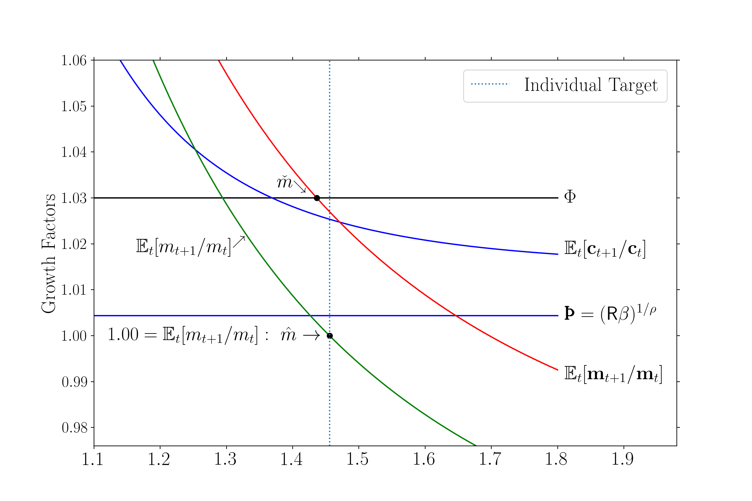
 Values and Expected Growth Rates
 Approaches Infinity
 ); clearly
  , since allowing the possibility of future noncapital
income cannot reduce current consumption. Our imposition of the
, since allowing the possibility of future noncapital
income cannot reduce current consumption. Our imposition of the  , so this solution satisfies our definition of nondegeneracy, and because this solution
is always available it defines a lower bound on both the consumption and value
functions.
, so this solution satisfies our definition of nondegeneracy, and because this solution
is always available it defines a lower bound on both the consumption and value
functions.
 (
(

 , and the continuous differentiability and strict concavity of
 therefore implies

 or lower than
  . Figure

 :
:


 ),
), 

 which goes to zero as
  goes to infinity.
![ÞÞÞ ≤ mlitm↑∞ 𝔼t[ct+1 ∕ct] ≤ ÞÞÞ](BufferStockTheory457x.svg)
 in the perfect
foresight model.
in the perfect
foresight model.
 is
is

 we have


 approaches zero.
 we have

![[( c(ℛ a(m ))) ]
limmt ↓0 𝔼t ---t+κ1¯mt--t- 𝒢t+1](BufferStockTheory467x.svg) is
positive, and the last line follows because the minimum possible realization of
is
positive, and the last line follows because the minimum possible realization of  is
is  so the minimum possible value of expected next-period consumption is
positive.
so the minimum possible value of expected next-period consumption is
positive.
 such that if
  , then
 ![𝔼 [m ] = m
t t+1 t](BufferStockTheory473x.svg) .
Existence of such a target turns out to require the
.
Existence of such a target turns out to require the 
![𝔼t[mt+1 ∕mt] = 1 if mt = ˆm.](BufferStockTheory475x.svg)

![∀mt ∈ (0, ˆm), 𝔼t[mt+1 ] > mt
∀mt ∈ (mˆ, ∞ ), 𝔼t[mt+1 ] < mt.](BufferStockTheory477x.svg)
 , the implicit equation for
  is
is


 . For our model, Figure
  for which
![𝔼 [m ]∕m = 𝔼 [c ]∕c = 𝒢
t t+1 t t t+1 t](BufferStockTheory484x.svg) for an individual consumer. Nevertheless, the next
section will show that economies populated by heterogeneous collections of such
consumers can exhibit balanced growth in the aggregate, and in the cross-section of
households.
for an individual consumer. Nevertheless, the next
section will show that economies populated by heterogeneous collections of such
consumers can exhibit balanced growth in the aggregate, and in the cross-section of
households.
 such
that, for all
such
that, for all
 ,
, ![𝔼t [mt+1 ∕mt ] < 𝒢](BufferStockTheory487x.svg) , and conversely if
, and conversely if  then
then ![𝔼t [mt+1 ∕mt ] > 𝒢](BufferStockTheory489x.svg) .
.
 will be the
  at which
  growth matches
  :
:
![𝔼 [m ]∕m = 𝔼 [p ]∕p
t t+1 t t t+1 t
𝔼t[mt+1 𝒢 Ψt+1pt]∕(mtpt ) = 𝔼t[pt𝒢Ψt+1 ]∕pt
⌊ ⌋
⌈ ⌉
𝔼t Ψt+1 ((◟mt-−--c(mt)R-∕◝(◜𝒢Ψt+1-)) +-ξξξt+1)◞ ∕mt = 1
mt+1
⌊ ℛ ⌋
◜◞◟◝
𝔼t⌈ (ˇm − c(mˇ))R ∕𝒢 + Ψt+1ξξξt+1⌉ = ˇm
(ˇm − c(mˇ))ℛ + 1 = ˇm.](BufferStockTheory494x.svg)
 for
for
 .
.

![𝔼t[Ψt+1mt+1 ∕mt ] = 1 if mt = ˇm.](BufferStockTheory509x.svg)

![∀mt ∈ (0, ˇm ), 𝔼t[mt+1 ]∕mt > 𝒢
∀mt ∈ (ˇm, ∞ ), 𝔼t[mt+1 ]∕mt < 𝒢.](BufferStockTheory511x.svg)
![𝔼t[mt+1∕mt ]](BufferStockTheory512x.svg) or
or ![𝔼t[mt+1 Ψt+1∕mt ]](BufferStockTheory513x.svg)
![𝔼t[mt+1 − mt]](BufferStockTheory514x.svg) or
or ![𝔼t [mt+1 Ψt+1 − mt]](BufferStockTheory515x.svg)
 But No Target
 , (
, ( for
for ![ℛ¯ = ℛ 𝔼 [Ψ −1]](BufferStockTheory520x.svg) , if there are no permanent shocks
(
, if there are no permanent shocks
( ), the conditions are identical. For many parameterizations (e.g., under the
baseline parameter values used for constructing figure
), the conditions are identical. For many parameterizations (e.g., under the
baseline parameter values used for constructing figure  and
and  will not differ
much.
will not differ
much.

 GIC-Mod}: No Target Exists But SS Does
 . But the pseudo-steady-state still exists
because it turns off realizations of the permanent shock. It is tempting to conclude that the
reason target
. But the pseudo-steady-state still exists
because it turns off realizations of the permanent shock. It is tempting to conclude that the
reason target  does not exist is that the increase in the size of the shocks induces a
precautionary motive that increases the consumer’s effective patience. But that
interpretation is not correct when the
does not exist is that the increase in the size of the shocks induces a
precautionary motive that increases the consumer’s effective patience. But that
interpretation is not correct when the  to
to  which reflects the fact that
in the presence of uncertainty the expectation of the inverse of the growth factor
increases:
which reflects the fact that
in the presence of uncertainty the expectation of the inverse of the growth factor
increases:  . That is, in the limit as
  the increase in effective impatience
reflected in
the increase in effective impatience
reflected in  is entirely due to the certainty-equivalence growth adjustment,
not to a (limiting) change in precaution. In fact, the next section will show that
an aggregate balanced growth equilibrium will exist even when realizations of the
permanent shock are not turned off: The required condition for aggregate balanced
growth is the regular
is entirely due to the certainty-equivalence growth adjustment,
not to a (limiting) change in precaution. In fact, the next section will show that
an aggregate balanced growth equilibrium will exist even when realizations of the
permanent shock are not turned off: The required condition for aggregate balanced
growth is the regular  , with the entire population at
  , but then evolves
according to the model’s assumed dynamics between
, but then evolves
according to the model’s assumed dynamics between  and
and  . Equation (
 will match the growth factor for permanent income
  . It is true that
there will be people for whom
. It is true that
there will be people for whom  is boosted by a small draw of
  . But
their contribution to the
. But
their contribution to the  , so their
 is reweighted by an amount that exactly unwinds that divisor-boosting. This means that
it is possible for the consumption-to-permanent-income ratio for every consumer to be
small enough that their market resources ratio is expected to rise, and yet for the
economy as a whole to exhibit a balanced growth equilibrium with a finite aggregate
balanced growth steady state
is reweighted by an amount that exactly unwinds that divisor-boosting. This means that
it is possible for the consumption-to-permanent-income ratio for every consumer to be
small enough that their market resources ratio is expected to rise, and yet for the
economy as a whole to exhibit a balanced growth equilibrium with a finite aggregate
balanced growth steady state  (this is not numerically the same as the individual
 because the problem’s nonlinearities have consequences when
aggregated).
because the problem’s nonlinearities have consequences when
aggregated).![i ∈ [0,1 ]](BufferStockTheory544x.svg) .
.
 ,
,  , and
, and
 under the condition
![GIC -Szeidl: log ÞÞÞ 𝒢 < 𝔼 [logΨ ]](BufferStockTheory549x.svg)
 ), but weaker than our
  ).
). as aggregate noncapital income in the long run (with
the corollary that aggregate assets and market resources grow at that same rate).
as aggregate noncapital income in the long run (with
the corollary that aggregate assets and market resources grow at that same rate). ![𝕄 [∙ ]](BufferStockTheory555x.svg) to yield the mean of its argument in the population (as distinct from
the expectations operator
to yield the mean of its argument in the population (as distinct from
the expectations operator ![𝔼[∙]](BufferStockTheory556x.svg) which represents beliefs about the future). Using
boldface capitals for aggregates, the growth factor for aggregate noncapital income
is:
which represents beliefs about the future). Using
boldface capitals for aggregates, the growth factor for aggregate noncapital income
is:

 and
and  .
.
 that we can consider it as Szeidl-converged. In such an
economy a microeconomist with a population-representative panel dataset could
calculate the growth rate of consumption for each individual household, and take the
average:
that we can consider it as Szeidl-converged. In such an
economy a microeconomist with a population-representative panel dataset could
calculate the growth rate of consumption for each individual household, and take the
average:
![𝕄 [Δ logct+1] = 𝕄 [logct+1pt+1 − logctpt]
= 𝕄 [logpt+1 − log pt] + 𝕄 [logct+1 − logct].](BufferStockTheory561x.svg)
 and
and  will be identical, so
that the second term in (
will be identical, so
that the second term in (![𝕄 [Δ logc ] = 𝕄 [Δ logp ] = log 𝒢.
t+1 t+1](BufferStockTheory564x.svg)
 . This fact is one way of interpreting Harmenberg’s
definition of the density of the permanent-income-invariant distribution of
. This fact is one way of interpreting Harmenberg’s
definition of the density of the permanent-income-invariant distribution of  ; call this
density
; call this
density  .
. the total amount of consumption at date
  by persons with market resources
 , and note that in the invariant economy this is given by the converged consumption
function
, and note that in the invariant economy this is given by the converged consumption
function  multiplied by the amount of permanent income accruing to such people
 . Since
  is invariant and aggregate permanent income grows according to
 , for any
  :
:

 and the
idiosyncratic component of permanent income
and the
idiosyncratic component of permanent income  does not shrink to zero; thus, covariances
are another potential measurement for construction of microfoundations.
does not shrink to zero; thus, covariances
are another potential measurement for construction of microfoundations.
 Harmenberg-converged economy, and define the mean value of the
consumption ratio as
Harmenberg-converged economy, and define the mean value of the
consumption ratio as ![𝔠t+n ≡ 𝕄 [ct+n]](BufferStockTheory581x.svg) . Normalizing period-
. Normalizing period- aggregate permanent income to
 , total consumption at
  and
and  are
are
![Ct+1 = 𝕄 [ct+1pt+1] = 𝔠t+1𝒢1 + covt+1 (ct+1,pt+1)
2
Ct+2 = 𝕄 [ct+2pt+2] = 𝔠t+2𝒢 + covt+2 (ct+2,pt+2)](BufferStockTheory586x.svg)
 allows us to obtain:

 , so the economy exhibits balanced growth in the
covariance:
, so the economy exhibits balanced growth in the
covariance:

 and the
  terms have constant growth factors
  and
and
 ,
, :
:


 . The revised result just says that in the
Harmenberg case where the mean value
. The revised result just says that in the
Harmenberg case where the mean value  of the consumption ratio
  can grow, the
covariance must rise in proportion to any ongoing expansion of
can grow, the
covariance must rise in proportion to any ongoing expansion of  (as well as in proportion to
the growth in
(as well as in proportion to
the growth in  ).
).
 and probability of remaining alive (not dead) is
  , then the assumption
that no utility accrues after death makes the effective discount factor
, then the assumption
that no utility accrues after death makes the effective discount factor  while the enhancement to the rate of return from the annuity scheme yields an
effective interest factor
while the enhancement to the rate of return from the annuity scheme yields an
effective interest factor  (recall that because of white-noise mortality, the
average wealth of the two groups is identical). Combining these, the effective patience
factor in the new economy
(recall that because of white-noise mortality, the
average wealth of the two groups is identical). Combining these, the effective patience
factor in the new economy  is unchanged from its value in the infinite horizon
model:
is unchanged from its value in the infinite horizon
model:

 (principally, the
 ).
).
 is the probability of remaining
alive, the condition changes from the plain
is the probability of remaining
alive, the condition changes from the plain 
 Functions Exist, are Concave, and Differentible
 , we start with a definition. We will say that a function
  is
‘nice’ if it satisfies
is
‘nice’ if it satisfies
 is well-defined iff
 is strictly increasing
 is strictly concave
 is
is 

 .
.
 .)
.)
 is nice. Our objective is to show that this implies
  is also nice;
this is sufficient to establish that
is also nice;
this is sufficient to establish that  is nice by induction for all
  because
 and
and  is nice by inspection.
 as
as
![[ 1−ρ ]
𝔳t(a ) = β 𝔼t 𝒢t+1vt+1(ℛt+1a + ξξξt+1 ) .](BufferStockTheory632x.svg)
 will attain its minimum of zero and since
 , it is clear that
  and
and  . So
. So  is
well-defined iff
is
well-defined iff  ; it is similarly straightforward to show the other properties required for
 to be nice. (See
  as
as

 since
since  and
and  are both
  , and note that our problem’s value function
defined in (
, and note that our problem’s value function
defined in (
 is well-defined if and only if
  . Furthermore,
  ,
,
 ,
,  , and
, and  . It follows that the
  defined by


 and
and  are strictly concave, both
  and
and  are
strictly increasing. Since both
are
strictly increasing. Since both  and
and  are three times continuously differentiable,
using (
are three times continuously differentiable,
using ( is continuously differentiable and

 is twice continuously differentiable (as is
  )
(See Appendix
)
(See Appendix  is nice, since
  .
.
 is Twice Continuously Differentiable
 is
is  . Define
  as
as  . Since
 and
and  ,
,

 and
and  are continuous and increasing,
  and
and
 are satisfied. Then
  for
sufficiently small
for
sufficiently small  . Hence we obtain a well-defined equation:

 is well-defined and

 , which means
  exists. Since
  is
is  ,
,
 exists and is continuous.
  is differentiable because
  is
is  ,
,  is
is  and
and  .
.  is given by
![′′ a′t(m )𝔳′t′′(at) [u ′′(ct) + 𝔳′′t(at)] − 𝔳′′t(at)[c′tu′′′(ct) + a′t𝔳′′t′ (at)]
ct(m ) = ---------------------′′-------′′----2--------------------.
[u (ct) + 𝔳 t(at)]](BufferStockTheory697x.svg)
 is continuous,
  is also continuous.
 Is a Contraction Mapping
 satisfies all of Boyd’s conditions.
 maps from
  to
to  . A preliminary requirement is
therefore that
. A preliminary requirement is
therefore that  be continuous for any
  bounded
  ,
,  . This is not
difficult to show; see
. This is not
difficult to show; see 
 implies
  by
inspection.
by
inspection. . By definition,
![{ ( 1−ρ ) }
{ 𝒯0}(m ) = max ct---- + β0
t ct∈[κmt,¯κmt] 1 − ρ](BufferStockTheory716x.svg)
 . Thus, condition (2) will hold if
  is
is
 -bounded, which it is if we use the bounding function

 . The
proof will be more compact if we define
. The
proof will be more compact if we define  and
and  as the consumption and assets
functions
as the consumption and assets
functions and
and  and
and  as the functions associated with
  ; using this
notation, condition (3) can be rewritten
; using this
notation, condition (3) can be rewritten

 consumer to consume the amount that is optimal for the
 consumer, value for the
  consumer must decline (at least weakly). That
is,
consumer must decline (at least weakly). That
is,


 by
assumption.
by
assumption. and defining
  , this condition is

 ) can be rewritten
as:
) can be rewritten
as:
![[ 1−ρ 1−ρ] 1− ρ
η > β-𝔼t-𝒢-t+1-(ˆatℛt+1-+-ξξξt+1)----−--m-t--.
1 − ℶ](BufferStockTheory739x.svg)
 is an arbitrary constant that we can pick, the proof thus reduces to showing
that the numerator of (
is an arbitrary constant that we can pick, the proof thus reduces to showing
that the numerator of (![[ ] [ ]
(1 − ℘ )β 𝔼t 𝒢1t−+ρ1(ˆatℛt+1 + 𝜃𝜃𝜃t+1∕(1 − ℘ ))1−ρ + ℘β 𝔼t 𝒢1t−+ρ1(ˆatℛt+1 )1− ρ − m1t−ρ
[ 1−ρ 1−ρ]
≤(1 − ℘ )β 𝔼t 𝒢t+1((1 − ¯κ)mt ℛt+1 + 𝜃𝜃𝜃t+1∕(1 − ℘))
+ ℘ βR1−ρ((1 − ¯κ)mt )1− ρ − m1t−ρ
[ 1−ρ 1−ρ]
=(1 − ℘ )β 𝔼t 𝒢t+1((1 − ¯κ)mt ℛt+1 + 𝜃𝜃𝜃t+1∕(1 − ℘))
( ( 1∕ρ)1 −ρ )
1−ρ( 1− ρ 1∕ρ(Rβ)---- )
+ m t ℘ βR ℘ R − 1
( )
[ ] | (R β)1∕ρ |
=(1 − ℘ )β 𝔼t 𝒢1t−+ρ1((1 − ¯κ)mt ℛt+1 + 𝜃𝜃𝜃t+1∕(1 − ℘))1−ρ + m1−t ρ| ℘1∕ρ--------− 1|
( ◟----◝◜R---◞ )
<1 by WRIC
[ 1−ρ 1−ρ] ρ 1−ρ
<(1 − ℘ )β 𝔼t 𝒢t+1(𝜃𝜃𝜃∕(1 − ℘ )) = ℶ (1 − ℘) 𝜃𝜃𝜃- .](BufferStockTheory741x.svg)

 defines a contraction mapping under the conditions (
 and
and 
 we made the restriction
  . However, in
the discussion of the consumption function bounds, we showed only (in (
. However, in
the discussion of the consumption function bounds, we showed only (in ( . (The difference is in the presence or absence of time subscripts on the
MPC’s.) We have therefore not proven (yet) that the sequence of value functions (
. (The difference is in the presence or absence of time subscripts on the
MPC’s.) We have therefore not proven (yet) that the sequence of value functions ( with
with  and the
 (and in the second step the reversal of the inequality
occurs because we have assumed
(and in the second step the reversal of the inequality
occurs because we have assumed  so that we are exponentiating both sides by the
negative number
so that we are exponentiating both sides by the
negative number  ). To see that this is a weak condition, note that for small values of
  this expression can be further simplified using
  so that it
becomes
so that it
becomes

 and recalling that the
  , the expression on the LHS above is
  times the
  not far below 1 and parameter values such that
  , this condition is clearly
not very different from the
, this condition is clearly
not very different from the  bounded space with a
unique
bounded space with a
unique  . But since
  and
and  , it must be
the case that the
, it must be
the case that the  toward which these
  ’s are converging is the
  that was the endpoint of the contraction defined by our operator
  . Thus,
under our slightly stronger (but still quite weak) conditions, not only do the value
functions defined by (
. Thus,
under our slightly stronger (but still quite weak) conditions, not only do the value
functions defined by ( defined by
 .
.
 defines a contraction mapping in an
  -bounded space. We
now show that
-bounded space. We
now show that  also defines a contraction mapping in Euclidian space.
 the unique fixed point of the operator
  , since
  ,
,

 and
and  because
  and
and  are
in
are
in  . It follows that


 ,
,  . On the other hand,
  means
means  , in other words,
  . Inductively one gets
 . This means that
  is a decreasing sequence,
bounded below by
is a decreasing sequence,
bounded below by  .
.

 .
.
 of
of  converging to
 . By the definition of
  , we have
![1−ρ
u(cT−n(i)(m ))+ β 𝔼T −n(i)[𝒢T− n(i)+1vT −n(i)+1(m )]
1−ρ
≥ u(cT−n(i)) + β 𝔼T −n(i)[𝒢T− n(i)+1vT−n(i)+1(m )],](BufferStockTheory802x.svg)
![cT−n(i) ∈ [κm, ¯κm ]](BufferStockTheory803x.svg) . Now letting
. Now letting  go to infinity, it follows that the left hand
side converges to
go to infinity, it follows that the left hand
side converges to ![u(c∗) + β 𝔼t[𝒢1t−ρv (m )]](BufferStockTheory805x.svg) , and the right hand side converges to
, and the right hand side converges to
![u(c ) + β 𝔼 [𝒢1−ρv (m )]
T− n(i) t t](BufferStockTheory806x.svg) . So the limit of the preceding inequality as
. So the limit of the preceding inequality as  approaches
infinity implies
approaches
infinity implies
![u (c∗) + β 𝔼 [𝒢1−ρv(m )] ≥ u(c ) + β 𝔼 [𝒢1− ρv(m )].
t t+1 T−n(i) t t+1](BufferStockTheory808x.svg)
![{ }
c∗ ∈ argmax u (cT−n(i)) + β 𝔼t[𝒢1− ρv(m )]
cT−n(i)∈[κm,¯κm] t+1](BufferStockTheory809x.svg) . By the uniqueness of
. By the uniqueness of  ,
,
 .
.
 , this
appendix taxonomizes the varieties of the limiting consumption function
, this
appendix taxonomizes the varieties of the limiting consumption function  that arise
under various parametric conditions.
that arise
under various parametric conditions.


 ). Under
 because
  implies that spending
everything today (setting
implies that spending
everything today (setting  ) produces lower marginal utility than is
obtainable by reallocating a marginal unit of resources to the next period at return
) produces lower marginal utility than is
obtainable by reallocating a marginal unit of resources to the next period at return
 :
:
 for a constrained consumer with a finite horizon of
  periods, so for
  such a
consumer’s consumption function will be the same as for the unconstrained case examined in
the main text.
such a
consumer’s consumption function will be the same as for the unconstrained case examined in
the main text.
 ) while the finite human wealth condition
holds, the limiting value of this consumption function as
) while the finite human wealth condition
holds, the limiting value of this consumption function as  is the degenerate
function
is the degenerate
function


 so the
consumption function limits to either
so the
consumption function limits to either  or
or  depending on the
relative speeds with which the MPC approaches zero and human wealth approaches
depending on the
relative speeds with which the MPC approaches zero and human wealth approaches
 .
.

 from Equation (
 .
. the unconstrained consumer would choose to consume more
than
the unconstrained consumer would choose to consume more
than  ; for such
  , the constrained consumer is obliged to choose
 .
. the constraint will never bind and the consumer will choose to spend the
same amount as the unconstrained consumer,
the constraint will never bind and the consumer will choose to spend the
same amount as the unconstrained consumer,  .
.
 will desire to consume more than 1. Such a consumer will
be constrained, not only in period
will desire to consume more than 1. Such a consumer will
be constrained, not only in period  , but perpetually thereafter.
 as the
  such that an unconstrained consumer holding
  would
behave so as to arrive in period
would
behave so as to arrive in period  with
with  (with
(with  trivially equal to 0); for
example, a consumer with
trivially equal to 0); for
example, a consumer with  was on the ‘cusp’ of being constrained in period
  :
Had
:
Had  been infinitesimally smaller, the constraint would have been binding
(because the consumer would have desired, but been unable, to enter period
been infinitesimally smaller, the constraint would have been binding
(because the consumer would have desired, but been unable, to enter period  with
negative, not zero,
with
negative, not zero,  ). Given the
  (and
thereafter) with resources of
(and
thereafter) with resources of  : The consumer cannot spend more
(because constrained), and will not choose to spend less (because impatient), than
: The consumer cannot spend more
(because constrained), and will not choose to spend less (because impatient), than
 .
.
 as follows.
Maintaining the assumption that the constraint has never bound in the past,
as follows.
Maintaining the assumption that the constraint has never bound in the past,  must have
been growing according to
must have
been growing according to  , so consumption
  periods in the past must have
been
periods in the past must have
been

 until
until  can thus be computed as

 and
and  (the relevant time
horizon, because from
(the relevant time
horizon, because from  onward the consumer will be constrained and unable to access
post-
onward the consumer will be constrained and unable to access
post- income) is


 such that the consumer with
  would
unconstrainedly plan (in period
would
unconstrainedly plan (in period  ) to arrive in period
  with
with  :
:

 , consider the function
  defined by linearly connecting the
points
defined by linearly connecting the
points  for integer values of
  (and setting
  for
for  ). This
function will return, for any value of
). This
function will return, for any value of  , the optimal value of
  for a liquidity constrained
consumer with an infinite horizon. The function is piecewise linear with ‘kink points’ where
the slope discretely changes; for infinitesimal
for a liquidity constrained
consumer with an infinite horizon. The function is piecewise linear with ‘kink points’ where
the slope discretely changes; for infinitesimal  the MPC of a consumer with assets
 is discretely higher than for a consumer with assets
  because the
latter consumer will spread a marginal dollar over more periods before exhausting
it.
because the
latter consumer will spread a marginal dollar over more periods before exhausting
it.
 , we need
  to become arbitrarily large with
  .
That is, we need
.
That is, we need

 , in which case the second term in (
 , and (
 , this will hold iff the RIC holds,
  . But given that the
FHWC
. But given that the
FHWC  holds, the GIC is stronger (harder to satisfy) than the RIC; thus,
the FHWC and the GIC together imply the RIC, and so a well-defined solution exists.
Furthermore, in the limit as
holds, the GIC is stronger (harder to satisfy) than the RIC; thus,
the FHWC and the GIC together imply the RIC, and so a well-defined solution exists.
Furthermore, in the limit as  approaches infinity, the difference between the limiting
constrained consumption function and the unconstrained consumption function becomes
vanishingly small, because the date at which the constraint binds becomes arbitrarily
distant, so the effect of that constraint on current behavior shrinks to nothing. That
is,
approaches infinity, the difference between the limiting
constrained consumption function and the unconstrained consumption function becomes
vanishingly small, because the date at which the constraint binds becomes arbitrarily
distant, so the effect of that constraint on current behavior shrinks to nothing. That
is,


 . We can rearrange (
 and
and  the numerators
and denominators of both terms multiplying
the numerators
and denominators of both terms multiplying  can be seen transparently to be positive.
So, the terms multiplying
can be seen transparently to be positive.
So, the terms multiplying  in (75) will be positive if
 . The
combined limit will be
. The
combined limit will be  if the term involving
  goes to
  faster than the term
involving
faster than the term
involving  goes to
  ; that is, if
 term is increasing backward in time at rate
dominated in the limit by
term is increasing backward in time at rate
dominated in the limit by  while the
  term is increasing at a rate dominated by
 term and
 .
.
 , the limit of the
  in (
in (

 . (Figure
  ,
,  ,
,  ,
,  ; note that the horizontal axis is bank balances
 ; the part of the consumption function below the depicted points is uninteresting
—
; the part of the consumption function below the depicted points is uninteresting
—  — so not worth plotting).

 Function with
  FHWC and
  RIC
RIC . But even if the
 the level of consumption in the model with
uncertainty would eventually exceed the level of consumption in the absence of
uncertainty.
the level of consumption in the model with
uncertainty would eventually exceed the level of consumption in the absence of
uncertainty.

 . We will henceforth refer
to this as the problem of the ‘restrained’ consumer (and, to avoid a common confusion, we will
refer to the consumer as ‘constrained’ only in circumstances when the constraint is actually
binding).
. We will henceforth refer
to this as the problem of the ‘restrained’ consumer (and, to avoid a common confusion, we will
refer to the consumer as ‘constrained’ only in circumstances when the constraint is actually
binding).
 as
as  where we separate the arguments by a semicolon to distinguish between
 , which is a state variable, and
  , which is not. The proposition we wish to demonstrate
is
, which is not. The proposition we wish to demonstrate
is

 , then argue that the desired result
propagates to earlier periods. For simplicity, suppose that the interest, growth, and
time-preference factors are
, then argue that the desired result
propagates to earlier periods. For simplicity, suppose that the interest, growth, and
time-preference factors are  , and there are no permanent shocks,
 ; the results below are easily generalized to the full-fledged version of the
problem.
; the results below are easily generalized to the full-fledged version of the
problem.
 is given by
  (in practice, this will
be
(in practice, this will
be  ), consider the unrestrained optimization problem

 so the expected marginal
value of ending period
so the expected marginal
value of ending period  with assets
  can be defined as


 therefore answers the question “With what level of assets would the restrained
consumer like to end period
therefore answers the question “With what level of assets would the restrained
consumer like to end period  if the constraint
  did not exist?” (Note that
the restrained consumer’s income process remains different from the process for the
unrestrained consumer so long as
did not exist?” (Note that
the restrained consumer’s income process remains different from the process for the
unrestrained consumer so long as  .) The restrained consumer’s actual asset position
will be
.) The restrained consumer’s actual asset position
will be
![`aT−1(m ) = max [0,`a∗T−1(m )],](BufferStockTheory984x.svg)

 at which the constraint makes the transition between binding and
non-binding in period
at which the constraint makes the transition between binding and
non-binding in period  .
.
![[ ]
′ − ρ ∫ ¯𝜃𝜃𝜃 − ρ
𝔳T−1(a;℘ ) ≡ ℘a + (1 − ℘ ) (cT (a + 𝜃𝜃𝜃∕ (1 − ℘ ))) dℱ𝜃𝜃𝜃 ,
𝜃𝜃𝜃](BufferStockTheory988x.svg)

 . Now note that for any fixed
  ,
,  .
Since the LHS of (
.
Since the LHS of ( .
That is, for any fixed value of
.
That is, for any fixed value of  such that the consumer subject to the restraint would
voluntarily choose to end the period with positive assets, the level of end-of-period assets for
the unrestrained consumer approaches the level for the restrained consumer as
such that the consumer subject to the restraint would
voluntarily choose to end the period with positive assets, the level of end-of-period assets for
the unrestrained consumer approaches the level for the restrained consumer as  . With
the same
. With
the same  and the same
  , the consumers must have the same
  , so the consumption
functions are identical in the limit.
, so the consumption
functions are identical in the limit.
 for which the restrained consumer is constrained. It is
obvious that the baseline consumer will never choose
for which the restrained consumer is constrained. It is
obvious that the baseline consumer will never choose  because the first term in (
 , while
  is finite (the marginal value of end-of-period
assets approaches infinity as assets approach zero, but the marginal utility of consumption has
a finite limit for
is finite (the marginal value of end-of-period
assets approaches infinity as assets approach zero, but the marginal utility of consumption has
a finite limit for  ). The subtler question is whether it is possible to rule out strictly
positive
). The subtler question is whether it is possible to rule out strictly
positive  for the unrestrained consumer.
 , that the unrestrained consumer is
considering ending the period with any positive amount of assets
, that the unrestrained consumer is
considering ending the period with any positive amount of assets  . For
any such
. For
any such  we have that
  . But by assumption we are
considering a set of circumstances in which
. But by assumption we are
considering a set of circumstances in which  , and we showed earlier that
 . So, having assumed
  , we have proven that the
consumer would optimally choose
, we have proven that the
consumer would optimally choose  , which is a contradiction. A similar argument holds
for
, which is a contradiction. A similar argument holds
for  .
.
 ,
,  which is the period
  version of (
 consumption functions, backwards recursion of the same arguments demonstrates that the
limiting consumption functions in previous periods are also identical to the constrained
function.
consumption functions, backwards recursion of the same arguments demonstrates that the
limiting consumption functions in previous periods are also identical to the constrained
function.

 we can define
  and
and  and the Euler
equation (
and the Euler
equation (![⌊( ( ) ) − ρ⌋
◜----=mt+◞1◟𝒢t+1----◝
|| | Ra (m ) + 𝒢 ξξξ | | |
et(mt )−ρ = βR 𝔼t |||| et+1(mt+1) || --t---t-----t+1-t+1|| || ||
⌈( ( mt ) ) ⌉
ρ [ −ρ ]
= (1 − ℘ )βRm t 𝔼t (et+1(mt+1)mt+1 𝒢t+1) | ξξξt+1 > 0
[( ) −ρ ]
+ ℘βR1 −ρ𝔼t et+1(ℛt+1at (mt))mt-−--ct(mt-) | ξξξt+1 = 0 .
mt](BufferStockTheory1022x.svg)
 then
then
 . Since
  ,
, ![𝔼t[(et+1(mt+1 )mt+1𝒢t+1)− ρ | ξξξt+1 > 0 ]](BufferStockTheory1026x.svg) is contained within bounds defined by
is contained within bounds defined by  and
and
 both of which are finite numbers, implying that the
whole term multiplied by
both of which are finite numbers, implying that the
whole term multiplied by  goes to zero as
  goes to zero. As
  the
expectation in the other term goes to
the
expectation in the other term goes to  . (This follows from the strict
concavity and differentiability of the consumption function.) It follows that the limiting
. (This follows from the strict
concavity and differentiability of the consumption function.) It follows that the limiting
 satisfies
  . Exponentiating by
  , we can conclude
that
, we can conclude
that


 , iterating (
 the ‘limiting maximal MPC.’
 . If the
 the proportion of current and future consumption that will be
financed out of capital approaches 1. Thus, the terms involving
the proportion of current and future consumption that will be
financed out of capital approaches 1. Thus, the terms involving  in (
in (![[ ]
(mtet(mt ))−ρ = βR 𝔼t (et+1 (at(mt )ℛt+1) (Rat (mt)))−ρ](BufferStockTheory1045x.svg)
 , and
, and  so a further limit of the Euler equation is
 holds, then a recursive formula for the minimal marginal propensity to
consume is given by
holds, then a recursive formula for the minimal marginal propensity to
consume is given by

 is also an increasing convergent sequence, and we define

 and so the limiting MPC is
  .
.


![𝔼t[mt+1 ∕mt] = 1 if mt = ˆm.](BufferStockTheory1061x.svg)

![∀m ∈ (0, ˆm), 𝔼 [m ] > m
t t t+1 t
∀mt ∈ (mˆ, ∞ ), 𝔼t[mt+1 ] < mt.](BufferStockTheory1063x.svg)
![𝔼t[mt+1∕mt ]](BufferStockTheory1064x.svg)
![𝔼t[mt+1 ∕mt] = 1](BufferStockTheory1065x.svg)
![𝔼t[mt+1 ] − mt](BufferStockTheory1066x.svg) is monotonically decreasing
is monotonically decreasing![𝔼t[mt+1 ∕mt ]](BufferStockTheory1067x.svg)
 and
and  ; Theorem
  ,
,  . Since
  , even if
 takes on its minimum value of 0,
  , since both
  and
and  are strictly
positive. With
are strictly
positive. With  and
and  both strictly positive, the ratio
 ![𝔼t[mt+1 ∕mt ]](BufferStockTheory1079x.svg) inherits
continuity (and, for that matter, continuous differentiability) from the consumption
function.
inherits
continuity (and, for that matter, continuous differentiability) from the consumption
function.
![𝔼t[mt+1∕mt ] = 1](BufferStockTheory1080x.svg) .
.![𝔼t[mt+1∕mt ]](BufferStockTheory1081x.svg) (just proven)
(just proven)
![𝔼 [m ∕m ] < 1
t t+1 t](BufferStockTheory1082x.svg)
![𝔼t [mt+1 ∕mt ] > 1](BufferStockTheory1083x.svg)
 where
where ![𝔼t[mt+1 ∕mt] < 1](BufferStockTheory1085x.svg)
 from the RHS, establishes that
![[ ]
ℛt+1-(mt-−-c(mt-)) +-ξξξt+1
lmitm↑∞ 𝔼t [mt+1 ∕mt ] = mltim↑∞ 𝔼t m
t
= 𝔼t [(R ∕𝒢t+1)ÞÞÞR]
= 𝔼t [ÞÞÞ ∕𝒢t+1]
< 1](BufferStockTheory1087x.svg)
 (see equation (
 is
is ![ℛ¯ = 𝔼t [ℛt+1 ]](BufferStockTheory1090x.svg) . In the next step
of this proof, we will prove that the combination
. In the next step
of this proof, we will prove that the combination 
 .
.
![limm ↑∞ 𝔼t[mt+1∕mt ] < 1](BufferStockTheory1093x.svg) whether the
whether the  > 1 where
 ![𝔼 [m ∕m ] > 1
t t+1 t](BufferStockTheory1095x.svg)
 in Section
 ![𝔼t[mt+1 ]](BufferStockTheory1097x.svg) to
to  is unbounded above
as
is unbounded above
as  because
 ![limmt ↓0𝔼t [mt+1 ] > 0](BufferStockTheory1100x.svg) .
.
![𝔼t[mt+1 ∕mt]](BufferStockTheory1101x.svg) is continuous, and takes on values above and
below 1, there must be at least one point at which it is equal to one.
is continuous, and takes on values above and
below 1, there must be at least one point at which it is equal to one.
![𝔼t[mt+1] − mt](BufferStockTheory1102x.svg) is monotonically decreasing.
is monotonically decreasing.![ζζζ(m ) ≡ 𝔼 [m ] − m
t t t+1 t](BufferStockTheory1103x.svg) and note that
and note that
![ζζζ(mt) < 0 ↔ 𝔼t[mt+1∕mt ] < 1
ζζζ(m ) = 0 ↔ 𝔼 [m ∕m ] = 1
t t t+1 t
ζζζ(mt) > 0 ↔ 𝔼t[mt+1∕mt ] > 1,](BufferStockTheory1104x.svg)
 . Our goal is to prove that
  is strictly decreasing on
  using the
fact that
using the
fact that
![( ) [( ) ]
′ -d-- -d-- ( )
ζζζ(mt ) ≡ dm ζζζ(mt) = 𝔼t dm ℛt+1 (mt − c(mt )) + ξξξt+1 − mt
t ′t
= ℛ¯ (1 − c (mt)) − 1.](BufferStockTheory1108x.svg)
 is decreasing (but for different
reasons) whether the
is decreasing (but for different
reasons) whether the  . We show
at the bottom of Section
. We show
at the bottom of Section  so
that
so
that

 .
.

 . Concavity of the consumption
function means that
. Concavity of the consumption
function means that  is a decreasing function, so everywhere

 from (
![[ ]
¯ -R--
ℛ ≡ 𝔼t 𝒢 Ψ < 1.](BufferStockTheory1119x.svg)

 gives
gives


![𝔼 [Ψ m ∕m ] = 1 if m = ˇm.
t t+1 t+1 t t](BufferStockTheory1124x.svg)

![∀mt ∈ (0, ˇm ), 𝔼t[mt+1 ]∕mt > 𝒢
∀mt ∈ (ˇm, ∞ ), 𝔼t[mt+1 ]∕mt < 𝒢.](BufferStockTheory1126x.svg)
![𝔼t[Ψt+1mt+1 ∕mt ]](BufferStockTheory1127x.svg)
![𝔼t[Ψt+1mt+1 ∕mt ] = 1](BufferStockTheory1128x.svg)
![𝔼t[Ψt+1mt+1 − mt ]](BufferStockTheory1129x.svg) is monotonically decreasing
is monotonically decreasing , our proof in
 ![𝔼t[mt+1 ∕mt]](BufferStockTheory1131x.svg) implies existence and continuity of
implies existence and continuity of ![𝔼t[Ψt+1mt+1 ∕mt ]](BufferStockTheory1132x.svg) .
.
 , our proof in Subsection
 ![𝔼t[mt+1 ]](BufferStockTheory1134x.svg) to
to  is unbounded as
  implies that the ratio
 ![𝔼t [Ψt+1mt+1 ]](BufferStockTheory1137x.svg) to
to  is
unbounded as
is
unbounded as  .
.
 goes to infinity is most easily calculated by
modifying the steps for the prior theorem explicitly:
goes to infinity is most easily calculated by
modifying the steps for the prior theorem explicitly:
![[ ( ) ]
lim 𝔼 [Ψ m ∕m ] = lim 𝔼 𝒢t+1--(R∕𝒢t+1-)a-(mt-) +-ξξξt+1--∕𝒢--
mt↑∞ t t+1 t+1 t mt ↑∞ t mt
[ ]
= lim 𝔼 (R-∕𝒢)a(mt-) +-Ψt+1-ξξξt+1
mt ↑∞ t mt
[ (R∕𝒢 )a(m ) + 1]
= lim ----------t-----
mt ↑∞ mt
= (R ∕𝒢)ÞÞÞR
= ÞÞÞ 𝒢
< 1](BufferStockTheory1141x.svg)
![𝔼t[Ψt+1mt+1 ∕mt ]](BufferStockTheory1142x.svg) is continuous, and takes on
values above and below 1, there must be at least one point at which it is equal to
one.
is continuous, and takes on
values above and below 1, there must be at least one point at which it is equal to
one.
![𝔼t[Ψt+1mt+1 ] − mt](BufferStockTheory1143x.svg) is monotonically decreasing.
is monotonically decreasing.![ζζζ(mt ) ≡ 𝔼t[Ψt+1mt+1 ] − mt](BufferStockTheory1144x.svg) and note that
and note that
![ζζζ(mt ) < 0 ↔ 𝔼t [Ψt+1mt+1 ∕mt] < 1
ζζζ(mt ) = 0 ↔ 𝔼t [Ψt+1mt+1 ∕mt] = 1
ζζζ(mt ) > 0 ↔ 𝔼t [Ψt+1mt+1 ∕mt] > 1,](BufferStockTheory1145x.svg)
 . Our goal is to prove that
  is strictly decreasing on
  using the
fact that
using the
fact that
![( ) [( ) ]
′ -d-- -d-- ( )
ζζζ(mt ) ≡ dm ζζζ(mt) = 𝔼t dm ℛ (mt − c(mt )) + Ψt+1 ξξξt+1 − mt
t t ′
= (R ∕𝒢)(1 − c (mt)) − 1.](BufferStockTheory1149x.svg)
 is decreasing (but for different
reasons) whether the
is decreasing (but for different
reasons) whether the 
 . We show
at the bottom of Section
. We show
at the bottom of Section  so
that
so
that

 .
.

 , the permanent-income growth factor
  , and the riskfree interest
factor
, and the riskfree interest
factor  . The arrows represent imposition of the labeled inequality condition (like, the
uppermost arrow, pointing from
. The arrows represent imposition of the labeled inequality condition (like, the
uppermost arrow, pointing from  to
to  , reflects imposition of the
  are there to make the diagram
readable for someone who may not immediately remember terms and definitions from the
main text. (Such a reader might also want to be reminded that
are there to make the diagram
readable for someone who may not immediately remember terms and definitions from the
main text. (Such a reader might also want to be reminded that  and
and  are all in
  ,
and that
,
and that  ).
).
 node and impose the
  .
.
 directly (without imposing
  and
and  )
by following the downward-sloping diagonal arrow exiting
)
by following the downward-sloping diagonal arrow exiting  . Although alternate
routes from one node to another all justify the same core conclusion (
. Although alternate
routes from one node to another all justify the same core conclusion ( , in
this case),
, in
this case),  symbol in the center is meant to convey that these routes are not
identical in other respects. This notational convention is used in
symbol in the center is meant to convey that these routes are not
identical in other respects. This notational convention is used in  , would be represented by moving the
arrowhead from the bottom right to the top left of the line segment connecting
, would be represented by moving the
arrowhead from the bottom right to the top left of the line segment connecting  and
and
 .
.
 and then impose
  , that would reverse the arrow
connecting
, that would reverse the arrow
connecting  and
and  , but the
  node would then have no exiting arrows so no further
deductions could be made. However, if we
node would then have no exiting arrows so no further
deductions could be made. However, if we  (that is, if we imposed
  ),
that would take us to the
),
that would take us to the  node, and we could deduce
  . However, we would have
to stop traversing the diagram at this point, because the arrow exiting from the
. However, we would have
to stop traversing the diagram at this point, because the arrow exiting from the
 node points back to our starting point, which (if valid) would lead us to the
conclusion that
node points back to our starting point, which (if valid) would lead us to the
conclusion that  . Thus, the reversal of the two earlier conditions (imposition of
 and
and  ) requires us also to reverse the final condition, giving us
 .
.

 node, it is possible to derive
the
node, it is possible to derive
the 

 node, we can follow the imposition of the
  ) and then
  to reach the conclusion that
  .
Algebraically,
.
Algebraically,

 .
. 

 ) by the
  ) raised to the power
  , which is
negative since we imposed
, which is
negative since we imposed  .
.  so when

 .
.


 and
and 
 and
and  respectively for
  (the
average value of the consumption ratio) and
(the
average value of the consumption ratio) and  . In the case of a Szeidl-invariant
economy, the main text shows that these are
. In the case of a Szeidl-invariant
economy, the main text shows that these are  and
and  . If the economy is
Harmenberg- but not Szeidl-invariant, no proof is offered that these growth factors will be
constant.
. If the economy is
Harmenberg- but not Szeidl-invariant, no proof is offered that these growth factors will be
constant.
 and
and  Grow Linearly
 increases apparently linearly. The second figure shows that
 also increases apparently linearly. (These results are produced by the
notebook
also increases apparently linearly. (These results are produced by the
notebook 
 Appears to Grow Linearly
 Appears to Grow Linearly