A Gentle Introduction to HARK: Buffer Stock Saving

This notebook explores the behavior of a consumer identical to the perfect foresight consumer described in Gentle-Intro-To-HARK-PerfForesightCRRA except that now the model incorporates income uncertainty and (artificial) borrowing constraints.

# This cell has a bit of initial setup.
# Click the "Run" button immediately above the notebook in order to execute the contents of any cell
# WARNING: Each cell in the notebook relies upon results generated by previous cells
#   The most common problem beginners have is to execute a cell before all its predecessors
#   If you do this, you can restart the kernel (see the "Kernel" menu above) and start over
from HARK.ConsumptionSaving.ConsIndShockModel import IndShockConsumerType
from HARK.ConsumptionSaving.ConsIndShockModel import PerfForesightConsumerType
from HARK.utilities import plot_funcs
import matplotlib.pyplot as plt

import numpy as np
from copy import deepcopy


def mystr(number):
    return "{:.4f}".format(number)

The Consumer’s Problem with Transitory and Permanent Shocks¶

Mathematical Description¶

Our new type of consumer receives two income shocks at the beginning of each period. Permanent income would grow by a factor $\Gamma$ in the absence of any shock , but its growth is modified by a shock, $\psi_{t+1}$ :

\begin{align} P_{t+1} & = \Gamma P_{t}\psi_{t+1} \end{align}

(1)

whose expected (mean) value is $\mathbb{E}_{t}[\psi_{t+1}]=1$ . Actual income received $Y$ is equal to permanent income $P$ multiplied by a transitory shock $\theta$ :

\begin{align} Y_{t+1} & = \Gamma P_{t+1}\theta_{t+1} \end{align}

(2)

where again $\mathbb{E}_{t}[\theta_{t+1}] = 1$ .

As with the perfect foresight problem, this model can be rewritten in terms of normalized variables, e.g. the ratio of ‘market resources’ $M_{t}$ (wealth plus current income) to permanent income is $m_t \equiv M_t/P_t$ . (See here for the theory). In addition, lenders may set a limit on borrowing: The ratio $a_{t}$ of end-of-period assets to permanent income $A_t/P_t$ must be greater than $\underline{a} \leq 0$ . (So, if $\underline{a}=-0.3$ , the consumer cannot borrow more than 30 percent of their permanent income).

The consumer’s (normalized) problem turns out to be:

No such environment: eqnarray* at position 7: \begin{̲e̲q̲n̲a̲r̲r̲a̲y̲*̲}̲
v_t(m_t) &=& \…

\begin{eqnarray*}
v_t(m_t) &=& \max_{c_t} ~~u(c_t) + \beta  \mathbb{E} [(\Gamma_{t+1}\psi_{t+1})^{1-\rho} v_{t+1}(m_{t+1}) ], \\
 & \text{s.t.} & \\
a_t &=& m_t - c_t, \\
a_t &\geq& \underline{a}, \\
m_{t+1} &=& a_t  R/(\Gamma_{t+1} \psi_{t+1}) + \theta_{t+1}.
\end{eqnarray*}

For present purposes, we assume that the transitory and permanent shocks are independent. The permanent shock is assumed to be (approximately) lognormal, while the transitory shock has two components: A probability $\wp$ that the consumer is unemployed, in which case $\theta^{u}=\underline{\theta}$ , and a probability $(1-\wp)$ of a shock that is a lognormal with a mean chosen so that $\mathbb{E}_{t}[\theta_{t+n}]=1$ .

Representing the Income Shocks¶

Computers are discrete devices; even if somehow we knew with certainty that the transitory and permanent shocks were, say, continuously lognormally distributed, in order to be represented on a computer those distributions would need to be approximated by a finite set of points. A large literature in numerical computation explores ways to construct such approximations; probably the easiest discretization to understand is the equiprobable approximation, in which the continuous distribution is represented by a set of $N$ outcomes that are equally likely to occur.

In the case of a single variable (say, the permanent shock $\psi$ ), and when the number of equiprobable points is, say, 5, the procedure is to construct a list: $\psi^{0}$ is the mean value of the continuous $\psi$ given that the draw of $\psi$ is in the bottom 20 percent of the distribution of the continuous $\psi$ . $\psi^{1}$ is the mean value of $\psi$ given that the draw is between the 20th and 40th percentiles, and so on. Having constructed these, the approximation to the expectation of some expression $g(\psi)$ can be very quickly calculated by:

\mathbb{E}_{t}[g(\psi)] \equiv \int_{0}^{\infty} g(\psi) dF_{\psi} \approx (1/N) \sum_{i=0}^{N-1} g(\psi^{i}).

(4)

(For a graphical depiction of a particular instance of this, see SolvingMicroDSOPs/#discreteApprox.)

The New Parameters¶

In addition to the parameters required for the perfect foresight model (like the time preference factor $\beta$ ), under the assumptions above, we need to choose values for the following extra parameters that describe the income shock distribution and the artificial borrowing constraint.

Param	Description	Code	Value
$\underline{a}$	Artificial borrowing constraint	$\texttt{BoroCnstArt}$	0.0
$\sigma_\psi$	Underlying stdev of permanent income shocks	$\texttt{PermShkStd}$	0.1
$\sigma_\theta^{e}$	Underlying stdev of transitory income shocks	$\texttt{TranShkStd}$	0.1
$N_\psi$	Number of discrete permanent income shocks	$\texttt{PermShkCount}$	7
$N_\theta$	Number of discrete transitory income shocks	$\texttt{TranShkCount}$	7
$\wp$	Unemployment probability	$\texttt{UnempPrb}$	0.05
$\underline{\theta}$	Transitory shock when unemployed	$\texttt{IncUnemp}$	0.3

Representation in HARK¶

HARK agents with this kind of problem are instances of the class $\texttt{IndShockConsumerType}$ , which is constructed by “inheriting” the properties of the $\texttt{PerfForesightConsumerType}$ and then adding only the new information required:

# This cell defines a parameter dictionary for making an instance of IndShockConsumerType.


IndShockDictionary = {
    "PermShkStd": [
        0.1
    ],  # ... by specifying the new parameters for constructing the income process.
    "PermShkCount": 7,
    "TranShkStd": [0.1],
    "TranShkCount": 7,
    "UnempPrb": 0.05,
    # ... and income for unemployed people (30 percent of "permanent" income)
    "IncUnemp": 0.3,
    # ... and specifying the location of the borrowing constraint (0 means no borrowing is allowed)
    "BoroCnstArt": 0.0,
    "cycles": 0,  # signifies an infinite horizon solution (see below)
}

Other Attributes are Inherited from PerfForesightConsumerType¶

You can see all the attributes of an object in Python by using the dir() command. From the output of that command below, you can see that many of the model variables are now attributes of this object, along with many other attributes that are outside the scope of this tutorial.

pfc = PerfForesightConsumerType()
dir(pfc)

['AgentCount',
 'BoroCnstArt',
 'CRRA',
 'DiscFac',
 'LivPrb',
 'MaxKinks',
 'PerfMITShk',
 'PermGroFac',
 'PermGroFacAgg',
 'RNG',
 'Rfree',
 'T_age',
 'T_cycle',
 '__class__',
 '__delattr__',
 '__dict__',
 '__dir__',
 '__doc__',
 '__eq__',
 '__format__',
 '__ge__',
 '__getattribute__',
 '__getstate__',
 '__gt__',
 '__hash__',
 '__init__',
 '__init_subclass__',
 '__le__',
 '__lt__',
 '__module__',
 '__ne__',
 '__new__',
 '__reduce__',
 '__reduce_ex__',
 '__repr__',
 '__setattr__',
 '__sizeof__',
 '__str__',
 '__subclasshook__',
 '__weakref__',
 '_constructor_errors',
 '_missing_key_data',
 'add_to_time_inv',
 'add_to_time_vary',
 'assign_parameters',
 'bilt',
 'calc_impulse_response_manually',
 'calc_limiting_values',
 'calc_stable_points',
 'check_AIC',
 'check_FHWC',
 'check_FVAC',
 'check_GICRaw',
 'check_RIC',
 'check_conditions',
 'check_elements_of_time_vary_are_lists',
 'check_restrictions',
 'clear_history',
 'construct',
 'constructors',
 'controls',
 'cycles',
 'default_',
 'del_from_time_inv',
 'del_from_time_vary',
 'del_param',
 'describe',
 'describe_constructors',
 'describe_model',
 'describe_parameters',
 'distributions',
 'get_Rfree',
 'get_controls',
 'get_mortality',
 'get_parameter',
 'get_poststates',
 'get_shocks',
 'get_states',
 'history',
 'initialize_sim',
 'initialize_sym',
 'kLogInitMean',
 'kLogInitStd',
 'kNrmInitCount',
 'kNrmInitDstn',
 'log_condition_result',
 'make_basic_SSJ',
 'make_shock_history',
 'model_file',
 'newborn_init_history',
 'pLogInitMean',
 'pLogInitStd',
 'pLvlInitCount',
 'pLvlInitDstn',
 'parameters',
 'post_solve',
 'poststate_vars',
 'pre_solve',
 'pseudo_terminal',
 'quiet',
 'read_shocks',
 'read_shocks_from_history',
 'reset_rng',
 'seed',
 'shock_history',
 'shock_vars',
 'shock_vars_',
 'shocks',
 'sim_birth',
 'sim_death',
 'sim_one_period',
 'simulate',
 'simulation_defaults',
 'solution_terminal',
 'solve',
 'solve_one_period',
 'solving_defaults',
 'state_now',
 'state_prev',
 'state_vars',
 'symulate',
 'time_inv',
 'time_inv_',
 'time_vary',
 'time_vary_',
 'tolerance',
 'track_vars',
 'transition',
 'unpack',
 'update',
 'verbose']

In python terminology, IndShockConsumerType is a superclass of PerfForesightConsumerType. This means that it builds on the functionality of its parent type (including, for example, the definition of the utility function). You can find the superclasses of a type in Python using the __bases__ attribute:

IndShockConsumerType.__bases__

(HARK.ConsumptionSaving.ConsIndShockModel.PerfForesightConsumerType,)

# So, let's create an instance of the IndShockConsumerType
IndShockExample = IndShockConsumerType(**IndShockDictionary)

As before, we need to import the relevant subclass of $\texttt{AgentType}$ into our workspace, then create an instance by passing the dictionary to the class as if the class were a function.

The Discretized Probability Distribution¶

The scatterplot below shows how the discretized probability distribution is represented in HARK: The lognormal distribution is represented by a set of equiprobable point masses.

# Plot values for equiprobable distribution of permanent shocks

plt.scatter(IndShockExample.PermShkDstn[0].atoms, IndShockExample.PermShkDstn[0].pmv)
plt.xlabel("Value")
plt.ylabel("Probability Mass")
plt.show()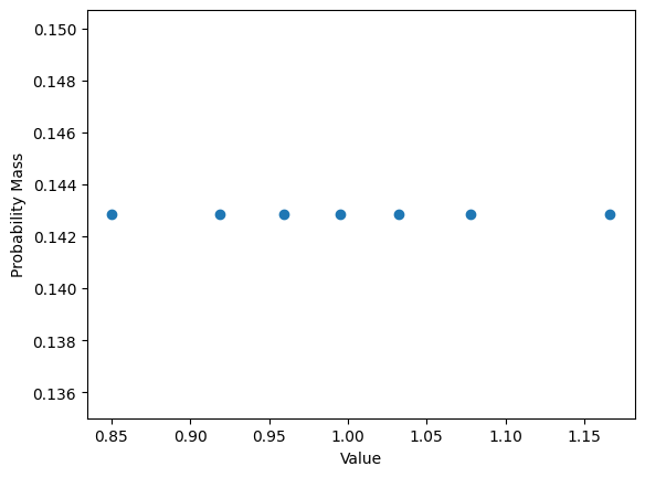

This distribution was created, using the parameters in the dictionary above, when the IndShockConsumerType object was initialized.

Solution by Backwards Induction¶

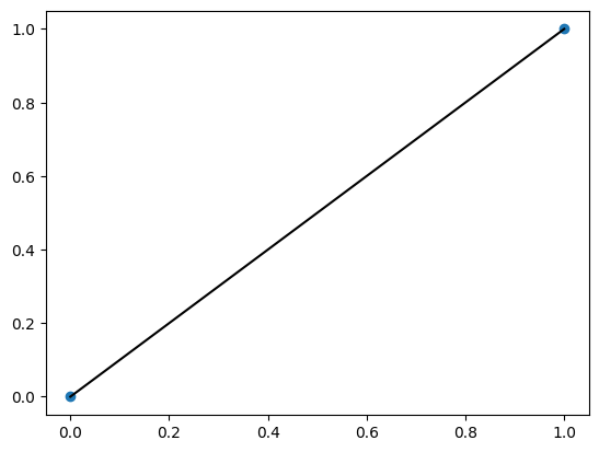
HARK solves this problem using backwards induction: It will derive a solution for each period ( $t$ ) by finding a mapping between specific values of market resources $\{m[0],m[1],...\}$ and the corresponding optimal consumption $\{c[0],c[1],...\}$ . The function that “connects the dots” will be stored in a variable named cFunc.

Backwards induction requires a “terminal” (last; final) period to work backwards from. IndShockExample constructed above did not specify a terminal consumption function, and consequently it uses the default terminal function in which all resources are consumed: $c_{T} = m_{t}$ .

IndShockExample.solution_terminal

<HARK.ConsumptionSaving.ConsIndShockModel.ConsumerSolution at 0x15aaad02d80>

The consumption function cFunc is defined by piecewise linear interpolation.

It is defined by a series of $(m,c)$ points on a grid; the value of the function for any $m$ is the $c$ determined by the line connecting the nearest defined gridpoints.

You can see below that in the terminal period, $c = m$ ; the agent consumes all available resources.

# Plot terminal consumption function
plt.plot(
    IndShockExample.solution_terminal.cFunc.x_list,
    IndShockExample.solution_terminal.cFunc.y_list,
    color="k",
)
plt.scatter(
    IndShockExample.solution_terminal.cFunc.x_list,
    IndShockExample.solution_terminal.cFunc.y_list,
)

The solution also has a representation of a value function, the value v(m) as a function of available market resources. Because the agent consumes all their resources in the last period, the value function for the terminal solution looks just like the CRRA utility function: $v_{T}(m) = u(m)$ .

# Final consumption function c=m
m = np.linspace(0.1, 1, 100)
plt.plot(m, IndShockExample.solution_terminal.vFunc(m))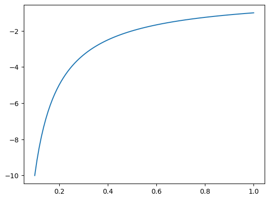

Solving the problem¶

This solution is generated by invoking solve() which is a method that is an attribute of the IndShockExample object. Methods in Python are supposed to have documentation that tell you what they do. You can read the documentation for methods and other attributes in HARK with the built-in Python help() function:

help(IndShockExample.solve)

Help on method solve in module HARK.core:

solve(verbose=False, presolve=True, postsolve=True, from_solution=None, from_t=None) method of HARK.ConsumptionSaving.ConsIndShockModel.IndShockConsumerType instance
    Solve the model for this instance of an agent type by backward induction.
    Loops through the sequence of one period problems, passing the solution
    from period t+1 to the problem for period t.

    Parameters
    ----------
    verbose : bool, optional
        If True, solution progress is printed to screen. Default False.
    presolve : bool, optional
        If True (default), the pre_solve method is run before solving.
    postsolve : bool, optional
        If True (default), the post_solve method is run after solving.
    from_solution: Solution
        If different from None, will be used as the starting point of backward
        induction, instead of self.solution_terminal.
    from_t : int or None
        If not None, indicates which period of the model the solver should start
        from. It should usually only be used in combination with from_solution.
        Stands for the time index that from_solution represents, and thus is
        only compatible with cycles=1 and will be reset to None otherwise.

    Returns
    -------
    none

Finite or Infinite Horizon?¶

$\texttt{ConsIndShockType}$ can solve either finite-horizon (e.g., life-cycle) problems, or infinite-horizon problems (where the problem is the same in every period). Elsewhere you can find documentation about the finite horizon solution; here we are interested in the infinite-horizon solution which is obtained (by definition) when iterating one more period yields a solution that is essentially the same. In the dictionary above we signaled to HARK that we want the infinite horizon solution by setting the “cycles” paramter to zero:

IndShockExample.cycles  # Infinite horizon solution is computed when cycles = 0

0

# Solve It
# Verbose prints progress as solution proceeds
IndShockExample.solve(verbose=True)

Finished cycle #1 in 0.001001596450805664 seconds, solution distance = 100.0
Finished cycle #2 in 0.0009992122650146484 seconds, solution distance = 10.088015890333434
Finished cycle #3 in 0.0009999275207519531 seconds, solution distance = 3.3534114736589693
Finished cycle #4 in 0.001001119613647461 seconds, solution distance = 1.6699529613894306
Finished cycle #5 in 0.00099945068359375 seconds, solution distance = 0.9967360674688486
Finished cycle #6 in 0.0009996891021728516 seconds, solution distance = 0.6602619046109499
Finished cycle #7 in 0.001001596450805664 seconds, solution distance = 0.4680948423143789
Finished cycle #8 in 0.0009999275207519531 seconds, solution distance = 0.34807706501006663
Finished cycle #9 in 0.0010120868682861328 seconds, solution distance = 0.2681341538834978
Finished cycle #10 in 0.0009875297546386719 seconds, solution distance = 0.21223248168627507
Finished cycle #11 in 0.0010097026824951172 seconds, solution distance = 0.17162798586899441
Finished cycle #12 in 0.0009918212890625 seconds, solution distance = 0.14121714401876462
Finished cycle #13 in 0.0010118484497070312 seconds, solution distance = 0.11786112023934692
Finished cycle #14 in 0.0009963512420654297 seconds, solution distance = 0.09954374358267515
Finished cycle #15 in 0.0 seconds, solution distance = 0.08492077965589839
Finished cycle #16 in 0.0009918212890625 seconds, solution distance = 0.07306820983636841
Finished cycle #17 in 0.0010006427764892578 seconds, solution distance = 0.06333371450893921
Finished cycle #18 in 0.0010001659393310547 seconds, solution distance = 0.055246317280595036
Finished cycle #19 in 0.0010123252868652344 seconds, solution distance = 0.04845886926538645
Finished cycle #20 in 0.0009996891021728516 seconds, solution distance = 0.04271110960013802
Finished cycle #21 in 0.000989675521850586 seconds, solution distance = 0.03780486582230225
Finished cycle #22 in 0.0010111331939697266 seconds, solution distance = 0.03358704056809492
Finished cycle #23 in 0.0009970664978027344 seconds, solution distance = 0.02993783577570497
Finished cycle #24 in 0.001003265380859375 seconds, solution distance = 0.026762425833982917
Finished cycle #25 in 0.0009882450103759766 seconds, solution distance = 0.02398495974448922
Finished cycle #26 in 0.0010004043579101562 seconds, solution distance = 0.02154418103929423
Finished cycle #27 in 0.0010120868682861328 seconds, solution distance = 0.019390181762538816
Finished cycle #28 in 0.0009992122650146484 seconds, solution distance = 0.017481967390489572
Finished cycle #29 in 0.0009980201721191406 seconds, solution distance = 0.015785611379662612
Finished cycle #30 in 0.0009908676147460938 seconds, solution distance = 0.014272839895086431
Finished cycle #31 in 0.0010135173797607422 seconds, solution distance = 0.012919936192925974
Finished cycle #32 in 0.00099945068359375 seconds, solution distance = 0.011706884785618321
Finished cycle #33 in 0.0009884834289550781 seconds, solution distance = 0.010616703056520294
Finished cycle #34 in 0.0 seconds, solution distance = 0.009634898474986997
Finished cycle #35 in 0.0010118484497070312 seconds, solution distance = 0.008749044420678587
Finished cycle #36 in 0.0009889602661132812 seconds, solution distance = 0.007948413988064118
Finished cycle #37 in 0.0009992122650146484 seconds, solution distance = 0.007223724470822646
Finished cycle #38 in 0.0010006427764892578 seconds, solution distance = 0.006566906564932307
Finished cycle #39 in 0.001009225845336914 seconds, solution distance = 0.005970916077072452
Finished cycle #40 in 0.0009906291961669922 seconds, solution distance = 0.005429579002498741
Finished cycle #41 in 0.0010123252868652344 seconds, solution distance = 0.004937463273915199
Finished cycle #42 in 0.0009887218475341797 seconds, solution distance = 0.004489772052600927
Finished cycle #43 in 0.0010120868682861328 seconds, solution distance = 0.00408225454644251
Finished cycle #44 in 0.0010004043579101562 seconds, solution distance = 0.0037111311701636396
Finished cycle #45 in 0.0010001659393310547 seconds, solution distance = 0.003373030500464669
Finished cycle #46 in 0.0 seconds, solution distance = 0.0030649359736796278
Finished cycle #47 in 0.0010001659393310547 seconds, solution distance = 0.0027841406665807256
Finished cycle #48 in 0.0010001659393310547 seconds, solution distance = 0.0025282088157077
Finished cycle #49 in 0.0009875297546386719 seconds, solution distance = 0.0022949429754119954
Finished cycle #50 in 0.0010008811950683594 seconds, solution distance = 0.0020823559119378388
Finished cycle #51 in 0.0009992122650146484 seconds, solution distance = 0.0018886464739757969
Finished cycle #52 in 0.001001596450805664 seconds, solution distance = 0.0017121788176552855
Finished cycle #53 in 0.001008749008178711 seconds, solution distance = 0.0015514644867233862
Finished cycle #54 in 0.0010004043579101562 seconds, solution distance = 0.0014051468883913287
Finished cycle #55 in 0.0009915828704833984 seconds, solution distance = 0.0012719878080478253
Finished cycle #56 in 0.0010118484497070312 seconds, solution distance = 0.0011508556554602478
Finished cycle #57 in 0.0009963512420654297 seconds, solution distance = 0.0010407151830378325
Finished cycle #58 in 0.0009918212890625 seconds, solution distance = 0.0009406184572169352
Finished cycle #59 in 0.0010008811950683594 seconds, solution distance = 0.0008496968979514463
Finished cycle #60 in 0.0 seconds, solution distance = 0.000767154229857514
Finished cycle #61 in 0.002000570297241211 seconds, solution distance = 0.0006922602130678968
Finished cycle #62 in 0.0 seconds, solution distance = 0.000624345042195884
Finished cycle #63 in 0.00119781494140625 seconds, solution distance = 0.0005627943195669616
Finished cycle #64 in 0.0008139610290527344 seconds, solution distance = 0.0005070445234864884
Finished cycle #65 in 0.0010004043579101562 seconds, solution distance = 0.0004565789051689251
Finished cycle #66 in 0.0009992122650146484 seconds, solution distance = 0.0004109237583840297
Finished cycle #67 in 0.0009894371032714844 seconds, solution distance = 0.00036964501506320246
Finished cycle #68 in 0.0010018348693847656 seconds, solution distance = 0.00033234512761959323
Finished cycle #69 in 0.0010101795196533203 seconds, solution distance = 0.0002986602050079057
Finished cycle #70 in 0.0010004043579101562 seconds, solution distance = 0.0002682573749837047
Finished cycle #71 in 0.0010020732879638672 seconds, solution distance = 0.00024083234929284103
Finished cycle #72 in 0.0010001659393310547 seconds, solution distance = 0.00021610717220754694
Finished cycle #73 in 0.0 seconds, solution distance = 0.0001938281357389826
Finished cycle #74 in 0.0009982585906982422 seconds, solution distance = 0.0001737638473713332
Finished cycle #75 in 0.001001596450805664 seconds, solution distance = 0.00015570343805260123
Finished cycle #76 in 0.0009987354278564453 seconds, solution distance = 0.00013945489982702952
Finished cycle #77 in 0.0009887218475341797 seconds, solution distance = 0.00012484354371933293
Finished cycle #78 in 0.001214742660522461 seconds, solution distance = 0.00011171056964087711
Finished cycle #79 in 0.0007989406585693359 seconds, solution distance = 9.991174074386322e-05
Finished cycle #80 in 0.0009884834289550781 seconds, solution distance = 8.931615549556682e-05
Finished cycle #81 in 0.0009989738464355469 seconds, solution distance = 7.980511119587419e-05
Finished cycle #82 in 0.0010004043579101562 seconds, solution distance = 7.12710531196592e-05
Finished cycle #83 in 0.0009999275207519531 seconds, solution distance = 6.361660386744461e-05
Finished cycle #84 in 0.0010137557983398438 seconds, solution distance = 5.675366786039859e-05
Finished cycle #85 in 0.0009870529174804688 seconds, solution distance = 5.060260605649347e-05
Finished cycle #86 in 0.0 seconds, solution distance = 4.5091476412739695e-05
Finished cycle #87 in 0.0020008087158203125 seconds, solution distance = 4.0155335675251536e-05
Finished cycle #88 in 0.0010001659393310547 seconds, solution distance = 3.573559836667073e-05
Finished cycle #89 in 0.0 seconds, solution distance = 3.1779449082502964e-05
Finished cycle #90 in 0.0010001659393310547 seconds, solution distance = 2.8239304256771902e-05
Finished cycle #91 in 0.0010006427764892578 seconds, solution distance = 2.507231993220671e-05
Finished cycle #92 in 0.0010135173797607422 seconds, solution distance = 2.2239942116364375e-05
Finished cycle #93 in 0.0009992122650146484 seconds, solution distance = 1.970749654489623e-05
Finished cycle #94 in 0.0009865760803222656 seconds, solution distance = 1.7443814823714376e-05
Finished cycle #95 in 0.001009225845336914 seconds, solution distance = 1.54208941594014e-05
Finished cycle #96 in 0.0009996891021728516 seconds, solution distance = 1.3613587938721139e-05
Finished cycle #97 in 0.0 seconds, solution distance = 1.1999324726730265e-05
Finished cycle #98 in 0.00199127197265625 seconds, solution distance = 1.0557853295622976e-05
Finished cycle #99 in 0.0010013580322265625 seconds, solution distance = 9.271011538913854e-06
Finished cycle #100 in 0.0010094642639160156 seconds, solution distance = 8.122517190400913e-06
Finished cycle #101 in 0.0 seconds, solution distance = 7.097778525810838e-06
Finished cycle #102 in 0.0012743473052978516 seconds, solution distance = 6.183723237906946e-06
Finished cycle #103 in 0.0007164478302001953 seconds, solution distance = 5.368643900993675e-06
Finished cycle #104 in 0.0010094642639160156 seconds, solution distance = 4.642058520687442e-06
Finished cycle #105 in 0.0010356903076171875 seconds, solution distance = 3.99458479938275e-06
Finished cycle #106 in 0.0009560585021972656 seconds, solution distance = 3.4178268535356437e-06
Finished cycle #107 in 0.0010089874267578125 seconds, solution distance = 2.9042732059281207e-06
Finished cycle #108 in 0.0009999275207519531 seconds, solution distance = 2.4472050079715757e-06
Finished cycle #109 in 0.0010004043579101562 seconds, solution distance = 2.0406135377015744e-06
Finished cycle #110 in 0.0010006427764892578 seconds, solution distance = 1.679126009790366e-06
Finished cycle #111 in 0.0009999275207519531 seconds, solution distance = 1.357939007018416e-06
Finished cycle #112 in 0.0009999275207519531 seconds, solution distance = 1.0727586712278026e-06
Finished cycle #113 in 0.0 seconds, solution distance = 8.19747068891985e-07

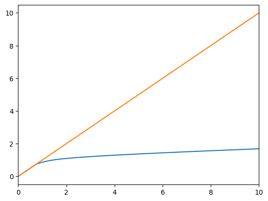
# plot_funcs([list],min,max) takes a [list] of functions and plots their values over a range from min to max
plot_funcs(
    [IndShockExample.solution[0].cFunc, IndShockExample.solution_terminal.cFunc],
    0.0,
    10.0,
)

Changing Constructed Attributes¶

In the parameter dictionary above, we chose values for HARK to use when constructing its numerical representation of $F_t$ , the joint distribution of permanent and transitory income shocks. When $\texttt{IndShockExample}$ was created, those parameters ( $\texttt{TranShkStd}$ , etc) were used by the constructor or initialization method of $\texttt{IndShockConsumerType}$ to construct an attribute called $\texttt{IncomeDstn}$ .

Suppose you were interested in changing (say) the amount of permanent income risk. From the section above, you might think that you could simply change the attribute $\texttt{TranShkStd}$ , solve the model again, and it would work.

That’s almost true-- there’s one extra step. $\texttt{TranShkStd}$ is a primitive input, but it’s not the thing you actually want to change. Changing $\texttt{TranShkStd}$ doesn’t actually update the income distribution... unless you tell it to (just like changing an agent’s preferences does not change the consumption function that was stored for the old set of parameters -- until you invoke the $\texttt{solve}$ method again). In the cell below, we invoke the method $\texttt{update\_income\_process}$ so HARK knows to reconstruct the attribute $\texttt{IncomeDstn}$ .

OtherExample = deepcopy(
    IndShockExample
)  # Make a copy so we can compare consumption functions
OtherExample.PermShkStd = [
    0.2
]  # Double permanent income risk (note that it's a one element list)
# Call the method to reconstruct the representation of F_t
OtherExample.update_income_process()
OtherExample.solve()

In the cell below, use your blossoming HARK skills to plot the consumption function for $\texttt{IndShockExample}$ and $\texttt{OtherExample}$ on the same figure.

# Use the remainder of this cell to plot the IndShockExample and OtherExample consumption functions against each other

Buffer Stock Saving?¶

There are some combinations of parameter values under which problems of the kind specified above have “degenerate” solutions; for example, if consumers are so patient that they always prefer deferring consumption to the future, the limiting consumption rule can be $c(m)=0$ .

The toolkit has built-in tests for a number of parametric conditions that can be shown to result in various characteristics in the optimal solution.

Perhaps the most interesting such condition is the “Growth Impatience Condition”: If this condition is satisfied, the consumer’s optimal behavior is to aim to achieve a “target” value of $m$ , to serve as a precautionary buffer against income shocks.

The tests can be invoked using the checkConditions() method:

IndShockExample.check_conditions(verbose=True)