¹Contact: ccarroll@jhu.edu, Department of Economics, 590 Wyman Hall, Johns Hopkins University, Baltimore, MD 21218, https://www.econ2.jhu.edu/people/ccarroll, and National Bureau of Economic Research.     ²Contact: lujan.14@osu.edu, Department of Economics, 410 Arps Hall, The Ohio State University, Columbus, OH 43220, https://economics.osu.edu.     ³Contact: mvelasq2@jhu.edu, Department of Economics, 590 Wyman Hall, Johns Hopkins University, Baltimore, MD 21218, https://www.econ2.jhu.edu.    

1 Introduction

Economists have long sought to use models of mathematically optimal behavior to try to understand saving and investment decisions over a household’s life-cycle¹ . If there were no uncertainty (about, say, investment returns), calculating optimal choices would not be hard. For example, consumers would want to invest their whole financial portfolio in whatever asset they knew (in advance) would yield the highest rate of return.

But in the real world, assets that – on average – yield higher returns (like stocks), also are much riskier than low-return safe assets (like bank deposits). Aversion to risk is a perfectly rational motivation, so how much to invest in risky versus safe assets is far from obvious. Furthermore, there are many other risks (to job, health, to house prices, and more) that should further temper any rational person’s appetite for risky investment.

As noted in Carroll (2020)² , calculating truly optimal behavior in a realistically uncertain world is such a difficult challenge that only recently has it become feasible to do with a reasonably high degree of realism. Rational choice models like the one we examined there must account for many important features of reality, including different types of uncertainty (labor income risk, mortality risk, and stock market risk), and should allow for reasonable choices of risk aversion, impatience, and other preferences. They need properly to account for for the path of income over the life cycle and into retirement, effects of aging and mortality, interest rates and economic growth, and myriad other factors.

All of this is so difficult that professional financial advisors do not attempt it, relying instead on rules of thumb and intuition to guide their clients. Indeed, despite the current excitement about the wonders of artificial intelligence, even online “robo-advisors” do not incorporate the degree of realism described above. Serious mathematical optimization efforts have been restricted to the pages of top academic economics journals – and the associated computer code used to solve the models in those papers has been so impenetrable as to be unusable.

Carroll (2020) described the first phase of our work sponsored by TFI in building a public, easy-to-use, open-source software toolkit of the computer code that can solve these kinds of problems. We showed that our free tools are able easily and quickly to reproduce the results that have been published in the academic literature.

However, as noted in Carroll (2020), those models of optimal decisionmaking imply that, given the robust rate of return that risky assets (’stocks’) have earned in the past, most consumers should invest all of their financial wealth in stocks over most of their lifetimes.

A tempting interpretation of the discrepancy between the models’ predictions and people’s actual choices is that most people are just making a mistake in not investing more in stocks. Another possibility, though, is that the models are still missing some vitally important (and rational) factor that weighs on people’s actual decisions; in this case, people might be making rational decisions and the models might be wrong.

There’s an obvious candidate for the missing factor. For most households homeownership is the biggest financial decision in their lives. Homeownership should matter for consumers’ choices about how willing they should rationally be to expose themselves to risky financial assets, for at least two reasons. First, homeownership exposes consumers to housing market price risk, which should have the effect of reducing their appetite for being exposed to other kinds of risk. Second, homeownership is associated with certain payment obligations (not just mortgages, but property taxes, maintenance costs, and so on), which reduces the flexibility they may have in adjusting their spending in response to income fluctuations.

These points may seem obvious, but there is a good reason they have not been incorporated in previous analyses of households’ optimal choice: Taking account of these complexities greatly increases the computational difficulty of calculating optimal decisions. This technical report describes results obtained using the latest tools to be added to the Econ-ARK toolkit; with these tools, it should be much easier for economists, financial planners, and others to understand the appropriate role of homeownership in modifying investors’ optimal saving and financial choices.

2 Literature Review

Beginning with Merton (1969) and Samuelson (1969), there is an extensive literature on portfolio choice over the life-cycle. Cocco, Gomes, and Maenhout (2005) develop a model of portfolio choice under incomplete markets and with labor income risk ³ . Although they are successful in solving a realistically calibrated life-cycle portfolio choice model, their results imply that most households, and in particular young households with low liquid wealth should invest all of their assets in the stock market. In reality, however, people choose a degree of stock market participation and risky share of assets much lower than what the model proposes would be optimal even for a person with very high risk aversion⁴ . This gap between observed and actual stock market participation is known as the stock market participation puzzle, and it remains an open question that is not explained by state-of-the-art quantitative life-cycle models.

One possible explanation for the stock market participation puzzle could be the absence of additional forms of asset holding and risk exposure that households face. In particular, housing has dual properties: Both as an asset and as a source of consumption services . Housing, however, is different from other assets in that it is illiquid and durable, providing both future expected wealth (house value of liquidation) as well as shelter as a consumption service. CHETTY, SÁNDOR, and SZEIDL (2017) empirically quantify the effect of housing on portfolio choice. Looking at the Survey of Income and Program Participation (SIPP) panel from 1990 to 2008, the authors establish the importance of property value and home equity (value minus mortgage debt) on stock market participation. Importantly, they find that a $10,000 increase in mortgage debt (holding home equity constant) causes the risky portfolio share to decrease by 0.6 percentage points or $275, which amounts to 3.9% of mean stockholdings in their data. Importantly for our purposes, they establish the need to distinguish the effects of home equity and mortgage debt in order to quantify the effect of housing on portfolios.

This project builds a quantitative model of housing and portfolio choice that can be used to interpret the empirical findings CHETTY, SÁNDOR, and SZEIDL (2017) in a rich framework that includes liquid wealth, illiquid housing (size and value), and mortgage debt, in order to capture the effects of home equity and mortgage debt on portfolio choice. While other recent work has attempted to shed light on this topic, this model is the first of its kind to explicitly track home value and mortgage debt separately, allowing them each to evolve with the decisionmaker’s choices and with economic shocks (say, to house prices). The 2-period model CHETTY, SÁNDOR, and SZEIDL (2017) develop misses the life-cycle properties of housing choice and income risk. Additionally, although their empirical findings reveal the importance of distinguishing home equity and mortgage debt, their model does not allow these variables to be chosen. Cocco (2005) and Yao and Zhang (2005) do allow choice of house size but do not distinguish between home equity and mortgage debt, instead only keeping track of net wealth as the total value of assets minus liabilities.

2.1 The House-Size Problem

When modeling housing decisions, different assumptions can be made about the “sizes” of houses that are available for people’s use. The “size” of a house is used to represent a scale of the different levels of utility that different houses yield, so a “big” house is simply a house that yields more utility than a “small” house. This section explores how the literature has dealt with the questions

• What kind of houses can people buy? Is there a finite number of types or a continuum of sizes?
• Can people change the size of their house without moving to a different house? are these changes continuous or lumpy? Are they decisions or are they mechanically tied to other life-cycle characteristics like permanent income?
• Do houses depreciate over time? Can this depreciation be offset?

In Cocco (2005) houses come in a continuum of sizes and once purchased, the houses’ sizes can not be changed. Agents can move to a different house of a whatever size they want every period, but must pay a transaction cost proportional to their current house’s price to do so. The total cost of moving to a size house from a size house is In this model, houses depreciate and agents must (exogenously) pay a cost each period to offset depreciation.

For Campbell and Cocco (2003), house sizes are exogenously set at the start of the agents’ lives and remain fixed for throughout their duration. The only “moving” that exists in the model is an exogenous event that can happen with a given probability in any period that forces the agent to sell his house, liquidate his mortgage and exit the model.There is no depreciation or associated costs.

Brandsaas (2018) develops a model where agents can rent or own their houses. Houses come in three fixed sizes; two for owners and one for renters . House sizes do not change, but agents can decide to move from one house size to another in any given period. Moving into a house entails a moving-cost (additional to the house’s purchase) that is proportional to the new house’s market value. Houses depreciate at a rate . To offset this, the owner must (exogenously) pay .

In Paz-Pardo (2021), agents can rent or own their houses. Houses come in three sizes: two for owning and one for renting (as in Brandsaas, 2018), and there is no depreciation. Agents can switch homes at any time but this entails a monetary cost that is proportional to the value of the new home. Agents also experience exogenous moving via a Calvo adjustment probability that forces homeowners to sell their house. Thereafter, households are forced to spend that period in a rented house.

3 Theoretical Framework

Perhaps the biggest financial decision in a household’s life is buying a house. Houses come in different sizes (and therefore costs), but they are generally an expensive asset whose value is at least a few times the household’s yearly income. Young households usually cannot buy their houses outright, as they start with little to no assets and take time to accumulate enough resources. They therefore usually rely on mortgages to purchase their houses. These young and leveraged households might thus be sensitive to stock market risk, causing them to reduce their stock market participation.

During the repayment period, households’ market resources (or liquid assets) are reduced by at least the fixed mortgage payment. This has two effects on risky asset choice: 1) It reduces ’market resources’ (current income, plus current non-housing wealth) today, making households relatively less wealthy, and 2) It reduces market resources in following periods for any given level of current savings, making households more risk averse due to the precautionary motive. The fixed nature of mortgage payments has another important effect: since the household must be sure to have sufficient resources in the next period to pay their mortgage and the cost of house maintenance, they might want to save more of their resources in a safe account rather than in the risky stock market.

Houses are also subject to price fluctuations that depend on local housing market conditions as well as broader national trends, such as recessions and expansions. The uncertain sale price of your house, then, constitutes additional uncertainty in future net worth and could thus have significant implications for portfolio decisions. One way to think about this is to realize that the owner of a house has an implicit holding of a risky asset, which should motivate them to want to reduce their exposure to additional risk in another risky asset, the stock market.

4 Methodology

The new model in our toolkit, which we call ConsPortfolioHousingModel, is an extension of the model we described in Carroll (2020), ConsPortfolioModel, with the added features of homeownership such as mortgage payments, house maintenance costs, and housing market price risk⁵ .

4.1 Young Households

The first stage of the model consists of young households making a decision to buy a house of fixed size. Importantly, young households have little to no assets and have recently joined the labor market, which means their income is also relatively small. In order to finance a home, then, young households must choose a house of a particular value and a corresponding mortgage size. Lenders are assumed to impose some microprudential conditions such as loan-to-income ratios to ensure that mortgages are repayable.

4.2 Mortgage payments

Once households choose a house and mortgage, they commit to fixed-rate payments for the rest of their working life, which is about 30 years. During this time, households have an implicit holding of a risky asset in their homes (because of their uncertain resale values), which may lead them to reduce their exposure to other risky assets, such as the stock market.

4.3 Retired homeowners

Once they reach retirement, households in our model have paid of their mortgage and have accumulated savings, making them significantly wealthier (where wealth here refers to their home equity and liquid assets) than young households. During this period, households experience a risk of house liquidation due to the possibility of being forced to move out due to poor health or old age. If they are forced to sell, they do so at their local housing market prices; the value of the house gets transformed into liquid wealth.

4.4 Retired renters

Retired renters have none of the complexities that come with owning a home, and thus behave like standard ConsPortfolioModel households. Instead of choosing only consumption, however, these households choose a level of total expenditures to spend on both consumption and rental housing. After becoming renters, households remain renters for the rest of their lives.

5 Results

5.1 Homeownership increases intensive margin of stock market participation

We examine here the behavior of retired households on the cusp of the liquidation of the value of their house. As usual, we are assuming that the household anticipates some form of guaranteed pension income (’Social Security’), but expects to finance any other consumption out of the returns on their assets.

The proportion of liquid assets invested in the stock market is known as the risky portfolio share, or risky share for short.

Carroll (2020) reviewed the logic of the model without housing. For a person with no housing wealth and little liquid wealth, the first dollar of investment in the stock market poses very little risk, so the model implies that the proportion of any additional wealth that will be invested in the stock market is 100 percent. But as wealth gets very large, the consumer becomes reluctant to put all of it in the stock market, because that would be putting more and more of their consumption at risk⁶ .

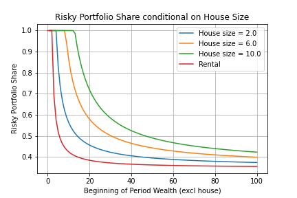
Figure 1 shows how the picture is modified for consumers who, in addition to their liquid assets, own homes of various sizes.

According to the model, retired households who own their homes and expect to sell them by next period have a higher risky share than retired households who rent, and their risky share increases with house size, holding liquid wealth constant.

Clearly, the bigger the house size, the wealthier the agents are in terms of net worth. In the standard portfolio choice model, wealthier households actually reduce their risky share to reduce risk in next period’s consumption. In the presence of housing, however, households still reduce their risk exposure as liquid wealth increases, but at a lower rate.

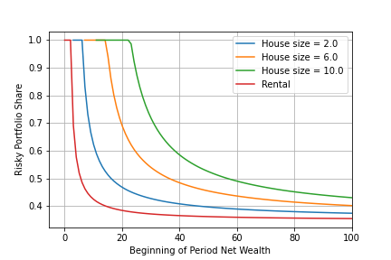
A better comparison is to add the expected value of the house to liquid wealth. In this way, we compare an agent with net worth with all liquid wealth and no home, with an agent with net worth, some of which is liquid wealth , and the rest is the illiquid expected house valuation , such that , where denotes house prices and represents the size of the agent’s house⁷ . As we see in figure 2, the increase in the risky portfolio share is more significant when considering home equity as part of net worth. Holding net wealth constant, households whose wealth is tied up in an illiquid asset have more risk appetite the larger the proportion of home equity to net wealth is.

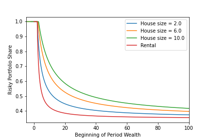
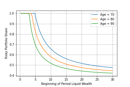
Additionally, an interesting observation is that according to the model retired households who are about to sell their homes are willing to risk at least the full home equity (expected value of their homes ) for certain when they have low liquidity. In other words, their risky share is equal to 1 at least up to the point where their liquid wealth is equal to their home equity. If we shift their liquid wealth leftward by the amount of their expected house valuation, we see in figure 3 that their risky share starts dropping at about the same point as it would if they rented a house instead. We can conclude that having a house shifts the risky share curve rightward by an amount equal to the home equity, but this is not the only effect. A larger house also reduces the rate at which the risky share decreases.

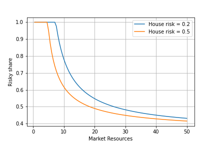
5.2 Increasing house price risk decreases risky share

The volatility of the housing market can have strong implications for the portfolio decisions of households who own their houses. A higher standard deviation in house prices implies a larger implicit holding of a risky asset (the house), regardless of house size. For this reason, households would optimally choose to avoid risk in other risky assets. As we see in figure 4 for 2 households who have a house of equal size, the risky share of a household in a more volatile market is lower than that of a household in a less volatile market, except at low levels of market resources. Households that experience high price volatility in the housing market reduce their exposure to risk elsewhere, leading to lower risky portfolio shares.

5.3 Larger houses increase households’ absolute risk taking

As mentioned before, a house represents an implicit holding in a risky market that is otherwise uncorrelated with the stock market. A larger house, however, provides a higher expected value of house liquidation which also means a higher expected future liquid wealth. Households with more valuable homes, then, have a higher absolute risk tolerance because their future housing value constitutes a buffer stock of wealth; thus they invest more resources in the risky asset market than they would if they had smaller homes. 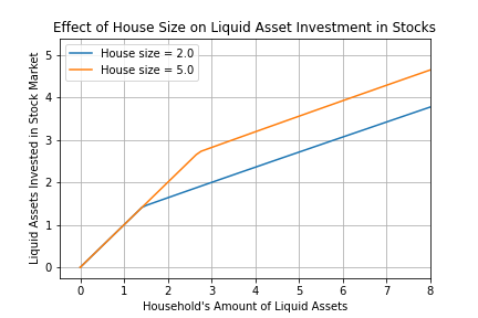In figure 5 we see that for an initial level of liquid assets, households of different house sizes invest the same amount of total assets in the stock market; this is the region where their risky share is 100%. Past this region, we see that households with a bigger house (and thus more home equity) are willing to invest a greater share of their liquid assets than peers with the same amount of liquid assets but less home equity. This indicates that home equity increases the level of risk appetite for households.

5.4 House size crowds out investment

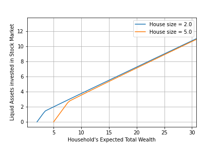
However, when comparing households on a total wealth basis, i.e. their liquid assets plus expected house liquidation, we can see that house size crowds out investment for households with low liquid wealth. In figure 6, we can consider a household whose house size is equal to 5 (5 times their yearly net income) and liquid assets are 0, so their total expected wealth is 5. As this household becomes wealthier, they invest all of their liquid assets in the stock market (such that their risky share is 100 percent), up to the point where they start rebalancing their portfolio between the risky and the safe asset. In this region, they are constrained from investing in the stock market by their low liquid wealth, as they surely would like to invest more in the market. This point becomes clearer by comparing the household to an equally wealthy peer with a smaller house. At the point where the household with house size of 5 has liquid wealth of 1 (1 times their yearly net income), they are investing less into the stock market in absolute terms than an equally wealthy household whose house size is equal to 2 and liquid assets are equal to 4. The total expected wealth of both these households is 6, but the household with the larger house is investing fewer assets in the stock market than the household with the smaller house. As their total wealth increases, however, both households are unconstrained by their house size and end up investing about the same amount into the stock market in absolute terms.

5.5 Optimal Portfolio Choice over the Lifecycle

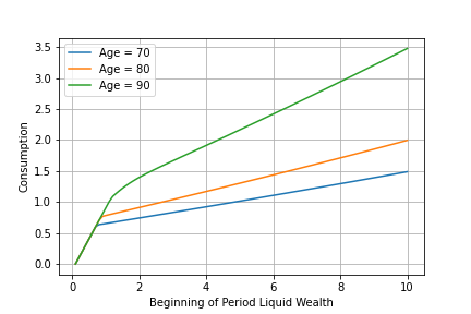
A result that is consistent with ConsPortfolioModel is that younger households have a higher risky share of assets than older households, when comparing households of equal house size and no mortgage debt. Similarly, older households consume more than younger households, as their consumption horizon gets shorter and the likelihood that they receive a windfall of wealth from their house liquidation increases.

6 Conclusions

Most people who need advice about how to invest in financial markets are also homeowners. But until now, even the most sophisticated and realistic analyses of how people should optimally invest in financial markets have not accounted for the (undeniably important) ramifications of homeownership for their financial choices.

That’s because constructing a model that correctly tracks all the potential interactions between homeownership, financial risk, and other kinds of risk is remarkably difficult. This report describes a free, publicly available open-source software tool that does these complex calculations. Sponsorship by the Think Forward Initiative has allowed us to add this tool to the free, open-source, Econ-ARK toolkit, thus making it available to financial institutions, financial planners, robo-advisors, academics, and anyone else who might be interested in a rigorous analysis of these questions.

Despite their combinatorial complexity, the answers that come from the model make intuitive sense. A first conclusion is that greater uncertainty about future house prices should make you less willing to invest in the stock market. In other words, a homeowner who lives in a place with wild house-price swings will find it best to have less exposure to other kinds of risk (like stock market risk) than someone with circumstances that are otherwise similar, but who lives in a place where house prices are more stable.

Another conclusion might seem to push in the other direction, but really does not: Among homeowners whose mortgage is paid off, for a given level of nonhousing net worth (say, $200K of financial assets net of mortgage debt), a person whose house is more valuable should invest more in risky financial asset. The reason is simple: For a given amount of liquid assets, the person with a bigger house is richer, and a richer person will want to have more money (in absolute terms) invested in the stock market).

The final point is that the existence of homeownership does not reverse one of the more surprising implications of the baseline model without homeownership: The richer you are, the lower is the optimal share of your portfolio in risky assets. This implication of the model does not match the available data well. The conclusion is easy to reverse by introducing a bequest motive in which bequests are a luxury good; but how exactly such a motive should be constructed is by no means a settled question, either among financial planners or among academic researchers. It is a topic we hope to address in future releases of our toolkit.

A The base model

At date 0, the household finances the purchase of a house with a mortgage loan. Given cash-on-hand at date 0 , which may come from previous savings or bequests, the household simultaneously chooses a house size (among a set of discrete house sizes) and a mortgage loan that meets the down-payment or Loan-to-Value requirement , where is the proportional down-payment, is the unit-price of housing, and is the chosen house size. An additional mortgage origination requirement observed in the literature is the Loan-to-Income ratio , which reflects initial mortgage affordability (Campbell and Cocco (2015)). Coincidentally, the household leaves some cash-on-hand to start next period with some liquidity.

(1)

A.1 Fixed-Rate Mortgage payments

When a household chooses a house size and mortgage loan, they also commit to a fixed payment amount and a loan duration of, for example, 30 years. To calculate the fixed rate mortgage payment (), we can start with the amount owed at the beginning of each period and subtract a fixed payment, which is then multiplied by a fixed mortgage interest rate . The limiting condition that ensures repayment at time is , which leads to as shown below:

(2)

where . Setting as a repayment requirement, the fixed rate mortgage payment is

(3)

The household is allowed to pay more than its required mortgage payment, which in this model leads to a decrease in the future minimum required payment to maintain the mortgage duration. If the household continually pays more than the minimum payment, becomes when the mortgage debt is fully paid off. This flexibility allows for the fixed rate mortgage payment to depend only on current mortgage debt and time to mortgage maturity, which is tracked by the age of the household .

A.2 The Investor’s problem in the presence of housing risk

A.2.1 Investing before Retirement

A working household begins period with cash-on-hand , housing size , mortgage debt , and permanent income . It must then choose a level of consumption , mortgage payment , and savings of which a fraction is invested into a risky asset and the rest into a safe asset.

The mortgage payment must be at least the fixed rate mortgage payment in order to ensure payoff within an expected maturity of years.

Although the model does not allow for explicit choices over housing adjustments, the household must nevertheless pay maintenance and upkeep costs due to housing depreciation at a cost of . Additionally, the household must also exogenously expand or contract their housing size given a life-cycle path of housing size . This parameter is intended to represent the observed path of the housing size component of portfolio compositions over the life-cycle.

(4)

A.2.2 Investing after Retirement

Households deterministically retire at age , and begin to experience exogenous risk of housing liquidation. By this time, the household has finished paying their mortgage debt, and so we lose the state variable. If the household is exogenously forced to liquidate their house, they receive their home equity at the beginning of next period and become renters until death. The problem of a household which faces housing risk is

(5)

The renter’s problem then becomes a simple portfolio problem where the household additionally pays for rental housing.

(6)

B Normalization

A useful strategy to facilitate finding the solution of these types of problems is normalization by permanent income. Throughout this section we assume

(7)

which is a Cobb-Douglas function nested inside a CRRA utility function. The model parameter determines the relative preference between non-durable consumption and housing size. In a simple rental housing problem, it also determines directly the rental housing share of total expenditures, as we’ll see below.

B.1 Rental Housing in the Utility

A renter pays for rental housing every period until death. Rental housing enters the utility as a non-durable expenditure and, like consumption, it has no impact on the continuation value. Using the utility function described above, and representing non-durable total expenditures as , utility maximization implies that , , and . Substituting these results into the utility function, it becomes:

(8)

Thus, we can represent the problem of total expenditures between consumption and rental housing as , where is a CRRA utility function with coefficient.

B.2 The Retired Renter’s last period of life

In the last period of life, a renter has no need to save and thus has to decide to spend all of his cash-on-hand () between non-durable consumption and rental housing.

(9)

Again, utility maximization implies that and . Substituting into the previous equation we obtain:

(10)

where . We can now normalize by permanent income such that lowercase variables are . Substituting , the expression becomes

(11)

If we define a normalized equation as then the original problem can be rewritten as

(12)

B.3 The Retired Renter’s second-to-last period

We can now consider the second-to-last period, although the same analysis will apply recursively to any period with a non-zero continuation value. Normalizing as above, where , we obtain

(13)

We can again define the normalized value function as and re-write the problem as

(14)

The generalized renter’s problem with non-zero continuation value then simplifies to a simple consumption and portfolio choice problem with additionally defined control variables as presented below.

(15)

B.4 The Retired Homeowner’s last period of life

We assume homeowners deterministically become renters before their last period of life.

B.5 The Retired Homeowner’s second-to-last period of life

In their second-to-last period of life, a homeowner will become a renter in the next period with certainty. Note that by this stage of life the household has no outstanding mortgage debt. Their problem is

(16)

A similar normalization procedure as above yields the following equivalent problem

(17)

B.6 The Retired Homeowner’s general problem

A retired homeowner has no mortgage debt or payments, but does experience house liquidation and house price risk. With probability , the homeowner will be forced to sell their house and become a renter next period, in which case they obtain the value of their home as a liquid asset.

(18)

The normalized version of their problem is

(19)

B.7 The Working Homeowner that has mortgage debt

B.8 The borrowing constraint

Every household arrives at the last period of the model as a retired renter. Because they will die with certainty by the end of the period, there is a strict no-borrowing constraint imposed for these households (). This implies that the minimum allowable level of market resources is also . If the household arrived to the last period with a negative level of market resources, it would have to consume a negative amount, yielding utility.

This strict borrowing constraint in the last period leads to a self imposed borrowing constraint in the second to last period, as the precautionary savings motive induces households to meet a minimum allowable level of market resources next period in order to avoid utility.

For the retired renter household, that means

(20)

Because renting households have no collateral (a home), we can assume an artificial no-borrowing constraint. The minimum allowable level of market resources next period is met as long as , which is true by construction. The no-borrowing constraint, in turn, induces a minimum allowable level of market resources in the second to last period as . Recursively, we can continue to assume a no-borrowing constraint for every period imposed on the retired renter household, which implies and for all during retirement.

The retired homeowner in their second to last period will become a renter with certainty by the next period, at which point they receive the cash value of their liquidated house.

(21)

which implies a natural minimum allowable level of market resources for homeowners of

(22)

The last period market resources for homeowners is ruled by the transition equation

(23)

Given a household’s decision on asset level , the lowest possible realization of next period market resources occurs when the household receives the lowest possible return, along with the lowest realizations of income shocks next period. For each , then, there is an upper bound on the risky share such that the minimum allowable level of future market resources is met.

(24)

which implies a natural risky share constraint of

(25)

The natural borrowing constraint, then, occurs when the implied natural risky share constraint is , which is

(26)

The minimum allowable level of market resources constraint is once again derived from the precautionary motive , which results in

(27)

An important issue arises in the third-to-last period. Households who will become renters next period only have to meet the minimum allowable level of market resources for rental households next period or equivalently . Households who will remain homeowners instead have to meet the minimum allowable level of market resources for home-owning households next period (determined above). However, unlike in the second-to-last period, households in the third-to-last period do not know what type they will be in the next period, so they must meet both constraints, and thus must meet the stricter constraint. The effective minimum allowable level of market resources for the second to-last-period and recursively for periods before it is:

(28)

and the general natural borrowing constraint for period and recursively for every period before it is

(29)

C Backsolving the problem

The overall return on the consumer’s portfolio is

(30)

The first order condition with respect to is

(31)

The first order condition with respect to is

(32)

A useful function to define is

(33)

with first order conditions

which implies first order conditions for the problem

We can define the problem

(38)

which leads to solution

(39)

we can solve for consumption function as

(40)

Similarly, as before, the Envelope condition is

(41)

D Portfolio Choice after retirement

D.1 The solution of risky share

Let be log-normally distributed such that , then it is true that

(42)

Thus, if we want to produce a log-normal distribution with mean and variance , we can use a normal distribution with

(43)

According to Campbell and Viceira, the optimal share of stocks in financial wealth for an agent that is not facing income uncertainty is

(44)

Using the above relations, we know that

(45)

D.2 Exogenous Risky Share

Given the solution of portfolio choice after retirement, if we want to target a particular risky share (for example, one that fits the observed data on portfolio choice after retirement), we can back out the agent’s beliefs on the risky asset return that would rationalize such an . Assuming we know an agent’s financial wealth (human and non-human), we can fix to find an ex-ante belief on the variance of the risky distribution that rationalizes an exogenous risky share as

(46)

Fixing and finding a that rationalizes an exogenous risky share has no analytical solution, although a numerical solution might exist under some conditions.

Of course, if instead we fix or , we can obtain rationalized beliefs as

(47)

and

(48)

It’s important to note that these beliefs will result in different risky distribution parameters than those that pegged the log-normal distribution parameter.

E The Portfolio Choice Problem for Rental Households

Households that do not own and instead rent their homes have to decide how much to consume, how much to spend on rent, and how much to save. Their normalized problem can be stated as:

(49)

Consider the problem of a consumer that has to spend on consumption and housing. Their problem is

(50)

Given the functional form of utility we are using (CRRA with paramter ), the well known solution to this simple problem is and . Restating the problem in terms of , we obtain:

(51)

where . Because both consumption and housing are non-durable in the case of a rental household, the consumer can first decide how much to spend on both goods () and then decide how much to spend on each of the goods without changing the problem. A further step to simplify the problem is to use iterated expectations to split up the problem into subperiods. We can define

(52)

Now, we can rewrite our original problem as

(53)

which embeds the simple subproblem and our defined iterated expectation.

We can rewrite the problem as

(54)

First order condition with respect to provides the Euler equation

(55)

and the first order condition with respect to is

(56)

The envelope condition is given by

(57)

And finally,

(58)

F The portfolio problem of a homeowner with no mortgage

A homeowner with no mortgage debt is allowed to invest more on their house to increase its size (or they can let it depreciate). In doing so, they choose home investment, consumption, and savings. Their problem is summarized as follows:

(59)

To facilitate the solution method, we can split the above problem into different subperiods.

In the first subperiod, the household arrives with cash on hand and their previous housing size. They then pick their current size by investing where housing costs are . After investing, they are left with net cash on hand after housing costs, and a new housing size.

(60)

In the second subperiod, the household arrives with net cash on hand and their current housing size. This subperiod is a standard portfolio choice problem, indexed by their house size. The agent must then choose a level of savings and the proportion of their savings that will go into the risky asset versus the safe asset .

(61)

Finally in the last subperiod, the household’s uncertainty is realized. Simultaneously, they observe their permanent and transitory income shocks, whether they will become renters in the next period (function with probability ), and if they do become renters, the liquidation price of their house per unit of housing.

(62)

F.1 First order conditions: Choosing home investment

The problem is

(63)

The first order condition with respect to is

(64)

which equalizes the marginal benefit of additional net cash-on-hand (cash-on-hand net of home investment) with the marginal cost of a larger house. The envelope conditions are

(65)

F.2 First order conditions: Choosing consumption and portfolio investment

Once again, let’s reduce the problem to 1 line.

(66)

Notice that passes through this problem unaltered. Indeed, in this subproblem, the house size indexes the portfolio choice (and may affect marginal utility) but does not need further addressing beyond a simple portfolio choice model.

The first order condition with respect to is

(67)

The first order condition with respect to is

(68)

Finally, the envelope conditions are

(69)

The second envelope condition is due to the nature of the pass-through.

F.3 Envelope conditions: Uncertainty is realized

The last subperiod is harder to re-write in one line, but because there is no maximization it is straight forward to calculate the derivatives.

(70)

G Solving the homeowner with mortgage problem

(71)

Can also be split up into subparts

(72)

(73)

(74)

References

Brandsaas, Eirik (2018): “Household Stock Market Participation: The Role of
Homeownership,” SSRN Electronic Journal.
Campbell, John Y., and João F. Cocco (2003): “Household risk
management and optimal mortgage choice,” Quarterly Journal of Economics, 118(4),
1449–1494.
__________ (2015): “A Model of Mortgage Default,” Journal of Finance, 70(4),
1495–1554.
Carroll, Christopher (2020): “Optimal Financial
Investments Over the Life Cycle,” Think Forward Initiative,
(https://www.thinkforwardinitiative.com/stories/optimal-financial-investments-over-the-life-cycle).
CHETTY, RAJ, LÁSZLÓ SÁNDOR, and ADAM SZEIDL (2017): “The
Effect of Housing on Portfolio Choice,” The Journal of Finance, 72(3), 1171–1212.
Cocco, João F. (2005): “Portfolio choice in the presence of housing,” Review of
Financial Studies, 18(2), 535–567.
Cocco, João F., F. J. Gomes, and Pascal J. Maenhout (2005):
“Consumption and portfolio choice over the life cycle,” Review of Financial Studies,
18(2), 491–533.
Gomes, Francisco (2020): “Portfolio Choice over the Life Cycle: A Survey,”
Annual Review of Financial Economics, 12(1), 277–304.
Gomes, Francisco, and Alexander Michaelides (2005): “Optimal life-cycle
asset allocation: Understanding the empirical evidence,” Journal of Finance, 60(2),
869–904.
Merton, Robert C. (1969): “Lifetime Portfolio Selection under Uncertainty: The
Continuous-Time Case,” The Review of Economics and Statistics, 51(3), 247.
Paz-Pardo, Gonzalo (2021): “Homeownership and Portfolio Choice over the
Generations,” Ssrn, pp. 1–87.
Samuelson, Paul A. (1969): “Lifetime Portfolio Selection By Dynamic Stochastic
Programming,” The Review of Economics and Statistics, 51(3), 239.
Yao, Rui, and Harold H. Zhang (2005): “Optimal consumption and portfolio
choices with risky housing and borrowing constraints,” Review of Financial Studies,
18(1), 197–239.
![[ ( )]
𝔳a = β 𝔼t Γ − ρRt+1 st∂mvH (mt+1, ht+1) + (1 − st)A˜∂mvR (mR ) (34)
t [ t+1 (t+1 t+1 t+1 ) ]
𝔳 ς = β 𝔼 Γ − ρ(R − R ) s ∂ vH (m ,h ) + (1 − s )A ˜∂ vR (mR ) a(35)
t t t+1 t+1 t m t+1 t+1 t+1 t m t+1 t+1 t](PortfolioChoiceWithRiskyHousing124x.svg)