Uninsured Idiosyncratic Risk and Aggregate Saving - Uninsured Idiosyncratic Risk and Aggregate Saving

Author: S. Rao Aiyagari

Quarterly Journal of Economics, 109(3):659–684

https://www.jstor.org/stable/2118417

Notebook by Adam Edwards

Introduction¶

Aiyigari’s 1994 paper introduces a Bewley model in which heterogenous agents face uninsurable idiosyncratic uncertainty in their income processes. Such uncertainty invokes precautionary saving on the part of the agents. Such models seek to examine the impact of uninsurable idiosyncratic risk on the saving behavior of agents, the aggregate saving rate, and inequality in wealth distributions.

Model¶

The model is characterized by the following:

\begin{split} &\max E_0\left(\sum_{t=0}^\infty \beta^t u(c_t)\right)\\ &\text{s.t.}\\ &c_t+a_{t+1}=w\ell_{t}+(1+r)a_t \\ &a_t\geq 0 \end{split}

(1)

where $\phi$ (if positive) is the limit on borrowing; $\ell_t$ is assumed to be an i.i.d labor endowment shock with bounded support given by $[\ell_{min},\ell_{max}]$ , $\ell_{min}>0$ ; and $w$ and $r$ represent the wage and interest rate repectively. The logarithm of the labor endowment shock follows an AR(1) process:

\begin{split} \log(\ell_t)=\rho\log(\ell_{t-1})+\sigma(1-\rho^2)^{\frac{1}{2}}\epsilon_{t}, \ \epsilon_t \sim N(0,1) \end{split}

(2)

The period utility function is assumed to be CRRA, $u(c) = \frac{c^{1-\mu} - 1}{1 - \mu}$ .

I wish to find a steady state of this economy; that is, for each combination of parameters, I want to find an interest rate $r$ such that the saving behavior induced by $r$ generates capital levels that imply rental rate $r$ . In other words, I am looking for a fixed point.

To illustrate, I will solve for the fixed point using the parameters of $\sigma = 0.2, \rho = 0.6, \mu = 3$ . First I import necessary packages.

import json
import os
import time
import warnings
import numpy as np
import matplotlib.pyplot as plt
import pandas as pd
from copy import deepcopy
from scipy.optimize import brentq

from HARK.ConsumptionSaving.ConsMarkovModel import MarkovConsumerType, markov_constructor_dict
from HARK.distributions import make_tauchen_ar1
from HARK.distributions import DiscreteDistributionLabeled
from HARK.utilities import plot_funcs

# Replaying a stored shock history, HARK warns that it does not store the aggregate
# productivity level PlvlAgg; that level is constant here (PermGroFacAgg = 1).
warnings.filterwarnings("ignore", message="The option for reading shocks was activated")

To begin tackling this problem I need to discretize the income process. Following Aiyagari, I will create a seven-state Markov chain using the Tauchen approximation to the AR1 process.

N = 7 # Number of income grid points
σ = 0.2
ρ = 0.6
μ = 3

shock_sd = lambda rho, sigma: sigma*(1-rho**2)**0.5

incomes, transition_matrix = make_tauchen_ar1(N, shock_sd(ρ, σ), ρ, 3)

Next, I will create a MarkovConsumerType with the desired parameters. The T and T_sum parameters define how many periods of the economy to simulate and to average over respectively.

T = 1000
T_sum = 700

AiyagariMarkovAgentDictionary = {
    "CRRA": 5.0,  # Coefficient of relative risk aversion
    "Rfree": [np.array(N * [1.03])],  # Interest factor on assets, for each labor endowment state
    "DiscFac": 0.96,  # Intertemporal discount factor
    "LivPrb": [np.array(N * [1.0])],  # Survival probability
    "AgentCount": 1000,  # Number of agents of this type (only matters for simulation)
    "kLogInitMean": 0.0,  # Mean of log initial assets (only matters for simulation)
    "kLogInitStd": 1.0,  # Standard deviation of log initial assets (only for simulation)
    "PermGroFacAgg": 1.0,  # Aggregate permanent income growth factor (only matters for simulation)
    "T_age": None,  # Age after which simulated agents are automatically killed
    "T_cycle": 1,  # Number of periods in the cycle for this agent type
    # Parameters for constructing the "assets above minimum" grid
    "aXtraMin": 0.001,  # Minimum end-of-period "assets above minimum" value
    "aXtraMax": 20,  # Maximum end-of-period "assets above minimum" value
    # Some other value of "assets above minimum" to add to the grid
    "aXtraExtra": np.array([0.005, 0.01]),
    "aXtraNestFac": 3,  # Exponential nesting factor when constructing "assets above minimum" grid
    "aXtraCount": 48,  # Number of points in the grid of "assets above minimum"
    "BoroCnstArt": 0.0,  # Artificial borrowing constraint; imposed minimum level of end-of period assets
    "CubicBool": False,  # Use cubic spline interpolation when True, linear interpolation when False
    "vFuncBool": False,  # Whether to calculate the value function during solution
    "global_markov": False,
    "cycles": 0,
    "PermGroFac": [
        np.array(N * [1.0])
    ],
    "MrkvPrbsInit": np.array(N * [1 / N]),  # Initial distribution of labor endowment states
    # The labor endowment process and its transition matrix are set below, so HARK's
    # constructors for them are switched off
    "constructors": {**markov_constructor_dict, "IncShkDstn": None, "MrkvArray": None},
}

AiyagariMarkovAgentDictionaryCopy = deepcopy(AiyagariMarkovAgentDictionary)
AiyagariMarkovAgentDictionaryCopy["CRRA"] = μ
AiyagariMarkovAgentDictionaryCopy["MrkvArray"] = [transition_matrix]
# This defines the labor endowments that the agents will be transitioning between
AiyagariMarkovAgentDictionaryCopy["IncShkDstn"] = [
    [DiscreteDistributionLabeled(pmv=np.ones(1), atoms=np.array([[1.0], [np.exp(x)]]), var_names=["PermShk", "TranShk"]) for x in incomes]
]

AiyagariMarkovType = MarkovConsumerType(**AiyagariMarkovAgentDictionaryCopy)
AiyagariMarkovType.T_sim = T
AiyagariMarkovType.track_vars = ["aNrm", "cNrm", "TranShk"]

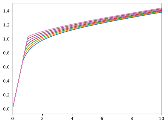
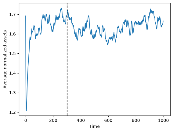
Now, simulate! First, I will input an interest rate of 3% and calculate the resulting capital levels. I display the consumption functions and then the average level of assets during the simulation.

R = 1.03
AiyagariMarkovType.Rfree = [np.array(N * [1.03])]

# Solve and simulate the agents
AiyagariMarkovType.solve()

print("Consumption function by labor endowment level:")
plot_funcs(AiyagariMarkovType.solution[0].cFunc, 0, 10)

Consumption function by labor endowment level:

AverageAggregateVar = lambda var: np.mean(np.sum(var[T-T_sum:T-1], axis=1))

AiyagariMarkovType.make_shock_history()
AiyagariMarkovType.initialize_sim()
AiyagariMarkovType.simulate()
plt.plot(np.mean(AiyagariMarkovType.history["aNrm"], axis=1));
plt.axvline(x = T - T_sum, color = 'k', linestyle = 'dashed');
plt.xlabel("Time");
plt.ylabel("Average normalized assets");
print("Calculated average normalized aggregate capital between T_sum and T:", AverageAggregateVar(AiyagariMarkovType.history["aNrm"]))

Calculated average normalized aggregate capital between T_sum and T: 1634.0803194370478

Here I define useful functions for the fixed point problem. As in Aiyagari (1994), I define the capital share to be 0.36 and depreciation rate to be 0.08.

α = 0.36
δ = 0.08
RFunc = lambda k : 1.0 + α * k ** (α - 1.0) - δ
wFunc = lambda k: (1.0 - α) * k ** (α)
RFunc_inv = lambda R : ((R - 1.0 + δ)/α)**(1.0/(α - 1.0))

# This function takes an interest rate, simulates an economy with such an interest rate, and calculates the interest rates implied by aggregate saving. 
def CalculateImpliedR(R):
    wRte = wFunc(RFunc_inv(R))

    # Give the agents the proposed interest factor and calculate wage rate
    AiyagariMarkovType.Rfree = [np.array(N * [R])]
    
    # Solve and simulate the agents
    AiyagariMarkovType.solve()
    AiyagariMarkovType.initialize_sim()
    AiyagariMarkovType.simulate()
    
    # Extract the agents' level of assets (capital holdings) and productivity at the end
    aNrm_agg = AverageAggregateVar(AiyagariMarkovType.history["aNrm"])
    pNrm_agg = AverageAggregateVar(AiyagariMarkovType.history["TranShk"])
    
    # Calculate aggregate capital and labor and take their ratio
    K = aNrm_agg*wRte # since assets are normalized, multiply by wage rate
    L = pNrm_agg
    k = K/L
    
    # Use the rule for determining Rfree to update the interest factor
    return RFunc(k)

def EquilibriumFunc(R):
    calculated = CalculateImpliedR(R)
    print("Input R:", R, "|| Implied R:", calculated, "|| Difference", calculated - R)
    return calculated - R

Now I can solve for the equilibrium interest rate. Since consumers cannot borrow, all of the capital stock comes from their saving, and all of the demand for capital comes from firms.

Solving for the equilibrium interest rate:

R_star = brentq(EquilibriumFunc, 0.99, 1.05)

Input R: 0.99 || Implied R: 1.3684749796221491 || Difference 0.37847497962214915

Input R: 1.05 || Implied R: 0.9345635966454547 || Difference -0.1154364033545453

Input R: 1.035976868644877 || Implied R: 1.0827521670188212 || Difference 0.04677529837394423

Input R: 1.0400205729293608 || Implied R: 1.012215646966888 || Difference -0.02780492596247286

Input R: 1.038513003070935 || Implied R: 1.0406506699575357 || Difference 0.0021376668866006643

Input R: 1.038620631765011 || Implied R: 1.0386517196399538 || Difference 3.10878749427701e-05

Input R: 1.0386222183233766 || Implied R: 1.0386221565430627 || Difference -6.178031397574557e-08

Input R: 1.0386222151766942 || Implied R: 1.0386222151785633 || Difference 1.8691714842589136e-12

Input R: 1.0386222151776947 || Implied R: 1.0386222151599187 || Difference -1.7776002891878306e-11

cNrm_agg = AverageAggregateVar(AiyagariMarkovType.history["cNrm"])
aNrm_agg = AverageAggregateVar(AiyagariMarkovType.history["aNrm"])
pNrm_agg = AverageAggregateVar(AiyagariMarkovType.history["TranShk"])

income = (R_star - 1.0 + δ)*aNrm_agg + pNrm_agg

saving = (1 - cNrm_agg/income)*100   #convert to %
saving_rate = float("%.2f" % saving)  #with 2 decimals

interest = (R_star - 1)*100
interest_rate = float("%.4f" % interest)  #with 4 decimals

print("σ:", σ, "ρ:", ρ, "μ:", μ, "|| Interest rate:", interest_rate, "|| Aggregate saving rate:", saving_rate)

σ: 0.2 ρ: 0.6 μ: 3 || Interest rate: 3.8622 || Aggregate saving rate: 24.33

This result is very similar to Aiyagari (1994), who calculates the interest rate and saving rate for this combination of parameters as 3.8767 and 24.25 respectively.

The baseline economy¶

The package aiyagari1994qje, in this repository’s src/, packages the computation above so that other programs can use it: other documents install it from GitHub and compute the same numbers. The cells below use it to describe the baseline economy ( $\sigma = 0.2$ , $\rho = 0.6$ , $\mu = 3$ ) at its equilibrium, after checking that it repeats the computation above exactly: the consumption functions, the distribution of wealth, and the supply of and demand for capital. Each figure is saved as PNG and SVG in baseline/, and every number, with the calibration and a definition of each, in baseline/numbers.json.

Quantities are in levels, for a population of mass one. The labor endowment in state $j$ is $\ell_j = \exp(x_j)$ , so aggregate labor supply $L$ , the population mean of $\ell$ , is about 1.02 rather than 1. HARK solves the household’s problem with the wage normalized to one; with wage $W$ , a household with market resources $m = (1+r)a + W\ell$ consumes $W c(m/W)$ , and its assets are $W$ times those of the normalized problem. Every statistic of the distribution comes from the simulation that determines the equilibrium: 1,000 households over the periods that AverageAggregateVar averages, pooled.

from aiyagari1994qje import Calibration, solve_equilibrium
from aiyagari1994qje import plot_capital_market, plot_consumption_functions, plot_wealth_lorenz

eq = solve_equilibrium(Calibration())
assert eq.interest_factor == R_star  # the package repeats the computation above exactly

print(f"Interest rate r* = {100 * eq.interest_rate:.4f}%; time-preference rate ϑ = {100 * eq.time_preference_rate:.4f}%")
print(f"Saving rate δK/Y = {100 * eq.saving_rate_from_capital:.2f}% (1 - C/Y in the simulation: {100 * eq.saving_rate:.2f}%); "
      f"with complete markets {100 * eq.saving_rate_complete_markets:.2f}%")
print(f"Labor supply L = {eq.labor_supply:.4f}; wage W = {eq.wage:.4f}")
print(f"Capital K* = {eq.capital:.4f}, against K^ϑ = {eq.capital_complete_markets:.4f} with complete markets: "
      f"{100 * (eq.capital / eq.capital_complete_markets - 1):.2f}% more")
print(f"Wealth Gini {eq.gini:.3f}; share of wealth held by the richest 1% {100 * eq.share_of_richest(0.01):.2f}%; "
      f"share of households at the borrowing constraint {100 * eq.share_at_borrowing_constraint:.2f}%")
print(f"Average MPC {eq.average_marginal_propensity_to_consume:.4f}; perfect-foresight MPC 1 - Þ_R = {1 - eq.return_patience_factor:.4f}")

os.makedirs("baseline", exist_ok=True)
plt.rcParams["svg.hashsalt"] = "Aiyagari1994QJE"  # fixed SVG element ids, so reruns write identical files

def save_figure(fig, name):
    # No timestamps or version stamps, so an unchanged figure is an unchanged file
    fig.savefig(f"baseline/{name}.png", dpi=200, bbox_inches="tight", metadata={"Software": None})
    fig.savefig(f"baseline/{name}.svg", bbox_inches="tight", metadata={"Creator": None, "Date": None})

Consumption functions. One for each labor endowment state, at the equilibrium interest rate. Below a kink, households consume all their market resources: they would like to borrow and cannot.

fig, ax = plt.subplots(figsize=(6.4, 4.8))
plot_consumption_functions(eq, ax)
save_figure(fig, "consumption-functions")
plt.show()

The distribution of wealth. The Lorenz curve of end-of-period assets, with the U.S. wealth shares that Krusell and Smith (1998, Table 1) report for the richest 1, 5, 10, 20 and 30 percent of households. Idiosyncratic labor income risk alone produces far less wealth inequality than the data show.

fig, ax = plt.subplots(figsize=(5, 5))
plot_wealth_lorenz(eq, ax)
save_figure(fig, "wealth-lorenz")
plt.show()

Supply of and demand for capital. Households supply capital by saving: at each interest rate, the supply is their average assets in the simulation. Firms demand capital until its marginal product net of depreciation equals the interest rate. As the interest rate approaches the time-preference rate $\vartheta = 1/\beta - 1$ , the supply grows without limit; with complete markets the economy would settle at $r = \vartheta$ with capital $K^\vartheta$ . Uninsurable risk makes households save more, so the equilibrium has more capital, $K^* > K^\vartheta$ , at a lower interest rate.

fig, ax = plt.subplots(figsize=(6.4, 4.8))
plot_capital_market(eq, ax)  # solves and simulates the economy at 48 interest rates
save_figure(fig, "capital-supply-demand")
plt.show()

The numbers. Everything above, with the calibration and a definition of each number, goes to baseline/numbers.json. Values are rounded to six significant digits.

numbers = eq.numbers()
numbers["figures"] = {
    "consumption-functions": "Consumption c against market resources m, one line per labor endowment state, at r*, "
                             "with the 45-degree line",
    "wealth-lorenz": "Lorenz curve of wealth, with the U.S. shares of the richest 1, 5, 10, 20 and 30 percent "
                     "(Krusell and Smith 1998, Table 1)",
    "capital-supply-demand": "Supply of capital (households' average assets) and demand for capital against the interest rate "
                             "in percent, the complete-markets line at the time-preference rate, and K* and K^ϑ marked",
}
with open("baseline/numbers.json", "w") as f:
    json.dump(numbers, f, indent=2, ensure_ascii=False)
    f.write("\n")
print(json.dumps({k: numbers[k] for k in ("equilibrium", "complete_markets", "wealth_distribution")}, indent=2, ensure_ascii=False))

Now to solve for equilibrium interest rates for all combinations of parameters:

σ_values = [0.2, 0.4]
ρ_values = [0.0, 0.3, 0.6, 0.9]
μ_values = [1, 3, 5]
results = []

index = 0
for σ in σ_values:  
    for ρ in ρ_values:
        for μ in μ_values:
            incomes, transition_matrix = make_tauchen_ar1(N, shock_sd(ρ, σ), ρ, 3)

            AiyagariMarkovAgentDictionaryCopy = deepcopy(AiyagariMarkovAgentDictionary)
            AiyagariMarkovAgentDictionaryCopy["CRRA"] = μ
            AiyagariMarkovAgentDictionaryCopy["MrkvArray"] = [transition_matrix]
            AiyagariMarkovAgentDictionaryCopy["IncShkDstn"] = [
                [DiscreteDistributionLabeled(pmv=np.ones(1), atoms=np.array([[1.0], [np.exp(x)]]), var_names=["PermShk", "TranShk"]) for x in incomes]
            ]

            AiyagariMarkovType = MarkovConsumerType(**AiyagariMarkovAgentDictionaryCopy)
            AiyagariMarkovType.T_sim = T
            AiyagariMarkovType.track_vars = ["aNrm", "cNrm", "TranShk"]

            print("σ:", σ, "ρ:", ρ, "μ:", μ)
            t = time.process_time()
            AiyagariMarkovType.make_shock_history()
            print("Time to generate shock history:", time.process_time() - t)

            R_star = brentq(EquilibriumFunc, 0.99, 1.05)

            cNrm_agg = AverageAggregateVar(AiyagariMarkovType.history["cNrm"])
            aNrm_agg = AverageAggregateVar(AiyagariMarkovType.history["aNrm"])
            pNrm_agg = AverageAggregateVar(AiyagariMarkovType.history["TranShk"])

            income = (R_star - 1.0 + δ)*aNrm_agg + pNrm_agg

            saving = (1 - cNrm_agg/income)*100   #convert to %
            saving_rate = float("%.2f" % saving)  #with 2 decimals

            interest = (R_star - 1)*100
            interest_rate = float("%.4f" % interest)  #with 4 decimals

            results.append([saving_rate, interest_rate])
            index = index + 1

            print("σ:", σ, "ρ:", ρ, "μ:", μ, "|| Interest rate:", interest_rate, "|| Aggregate saving rate:", saving_rate)
            print("")

σ: 0.2 ρ: 0.0 μ: 1

Time to generate shock history: 3.828915000000002

Input R: 0.99 || Implied R: 1.9837698242432893 || Difference 0.9937698242432893

Input R: 1.05 || Implied R: 0.920854202334329 || Difference -0.12914579766567102

Input R: 1.043099438899276 || Implied R: 0.9499624293592571 || Difference -0.09313700954001891

Input R: 1.0267805090471234 || Implied R: 1.572528047169771 || Difference 0.5457475381226475

Input R: 1.0407204545727913 || Implied R: 1.1484947639834655 || Difference 0.10777430941067423

Input R: 1.041996606629454 || Implied R: 0.9928439186718966 || Difference -0.04915268795755734

Input R: 1.041150205130333 || Implied R: 1.0971319278524572 || Difference 0.055981722722124205

Input R: 1.0416008950017943 || Implied R: 1.0338878682939183 || Difference -0.007713026707875992

Input R: 1.041536161354706 || Implied R: 1.0424728621394181 || Difference 0.0009367007847120856

Input R: 1.0415431715244572 || Implied R: 1.0415240851724894 || Difference -1.908635196778974e-05

Input R: 1.0415430315366272 || Implied R: 1.041542991047995 || Difference -4.048863222472221e-08

Input R: 1.041543031239047 || Implied R: 1.041543031239347 || Difference 2.999822612537173e-13

Input R: 1.0415430312400475 || Implied R: 1.0415430311042244 || Difference -1.3582313052040718e-10
σ: 0.2 ρ: 0.0 μ: 1 || Interest rate: 4.1543 || Aggregate saving rate: 23.85

σ: 0.2 ρ: 0.0 μ: 3

Time to generate shock history: 3.7599969999999985

Input R: 0.99 || Implied R: 1.4829122892954594 || Difference 0.4929122892954594

Input R: 1.05 || Implied R: 0.9352027032606937 || Difference -0.11479729673930639

Input R: 1.0386659056189969 || Implied R: 1.141033995452829 || Difference 0.10236808983383217

Input R: 1.0440086059916869 || Implied R: 0.9672320318095836 || Difference -0.07677657418210326

Input R: 1.041718868623567 || Implied R: 1.01693000762891 || Difference -0.024788860994656936

Input R: 1.0408399148722671 || Implied R: 1.0531005644803497 || Difference 0.012260649608082597

Input R: 1.0411307835987653 || Implied R: 1.0402633220999546 || Difference -0.0008674614988106732

Input R: 1.041111563970032 || Implied R: 1.0410911130248919 || Difference -2.0450945140026988e-05

Input R: 1.041111100687687 || Implied R: 1.0411111084230933 || Difference 7.735406315489968e-09

Input R: 1.0411111008628535 || Implied R: 1.0411111008624847 || Difference -3.68816088780477e-13

Input R: 1.041111100861853 || Implied R: 1.0411111009056717 || Difference 4.381872642511553e-11
σ: 0.2 ρ: 0.0 μ: 3 || Interest rate: 4.1111 || Aggregate saving rate: 23.92

σ: 0.2 ρ: 0.0 μ: 5

Time to generate shock history: 3.768706999999992

Input R: 0.99 || Implied R: 1.3539661658773678 || Difference 0.36396616587736785

Input R: 1.05 || Implied R: 0.9475976272851615 || Difference -0.10240237271483854

Input R: 1.0368255642170092 || Implied R: 1.1265278686265883 || Difference 0.08970230440957905

Input R: 1.042977300170137 || Implied R: 0.9910909750958089 || Difference -0.05188632507432811

Input R: 1.0407229456178055 || Implied R: 1.0336091737037483 || Difference -0.007113771914057265

Input R: 1.040391076822961 || Implied R: 1.0417909932547527 || Difference 0.0013999164317917145

Input R: 1.0404456464243168 || Implied R: 1.0404224204381334 || Difference -2.3225986183428304e-05

Input R: 1.0404447558368457 || Implied R: 1.0404446898375124 || Difference -6.599933333184538e-08

Input R: 1.040444753299046 || Implied R: 1.040444753298943 || Difference -1.0302869668521453e-13

Input R: 1.0404447532980454 || Implied R: 1.0404447533239647 || Difference 2.5919266732898905e-11
σ: 0.2 ρ: 0.0 μ: 5 || Interest rate: 4.0445 || Aggregate saving rate: 24.04

σ: 0.2 ρ: 0.3 μ: 1

Time to generate shock history: 3.8032089999999954

Input R: 0.99 || Implied R: 2.018727393794474 || Difference 1.028727393794474

Input R: 1.05 || Implied R: 0.9208573070498646 || Difference -0.12914269295013547

Input R: 1.0433079179903564 || Implied R: 0.9459233057713744 || Difference -0.09738461221898198

Input R: 1.0245615964704229 || Implied R: 1.5382913648119914 || Difference 0.5137297683415685

Input R: 1.0403205831970292 || Implied R: 1.12705054789323 || Difference 0.08672996469620076

Input R: 1.0417278125728997 || Implied R: 1.0045390415697142 || Difference -0.03718877100318552

Input R: 1.0413054944245355 || Implied R: 1.0425525466942387 || Difference 0.0012470522697032305

Input R: 1.0413191965586543 || Implied R: 1.041216302970888 || Difference -0.00010289358776627289

Input R: 1.0413181521747394 || Implied R: 1.0413180597447953 || Difference -9.242994414293548e-08

Input R: 1.041318151235789 || Implied R: 1.0413181512362122 || Difference 4.2321701698710967e-13

Input R: 1.0413181512367895 || Implied R: 1.0413181511387142 || Difference -9.807532563854693e-11
σ: 0.2 ρ: 0.3 μ: 1 || Interest rate: 4.1318 || Aggregate saving rate: 23.85

σ: 0.2 ρ: 0.3 μ: 3

Time to generate shock history: 3.7839560000000034

Input R: 0.99 || Implied R: 1.4166035804138741 || Difference 0.42660358041387414

Input R: 1.05 || Implied R: 0.9350020624840051 || Difference -0.11499793751599496

Input R: 1.0372602346512383 || Implied R: 1.12023022176166 || Difference 0.0829699871104217

Input R: 1.0425995751972952 || Implied R: 0.9829694606330489 || Difference -0.05963011456424627

Input R: 1.0403668594788642 || Implied R: 1.038403275276933 || Difference -0.001963584201931212

Input R: 1.0402925916421184 || Implied R: 1.0406639781472011 || Difference 0.00037138650508272697

Input R: 1.0403044042409857 || Implied R: 1.0403039933809286 || Difference -4.1086005708734774e-07

Input R: 1.0403043911873024 || Implied R: 1.0403043911079006 || Difference -7.940181845356165e-11

Input R: 1.0403043911847791 || Implied R: 1.0403043911847825 || Difference 3.3306690738754696e-15

Input R: 1.0403043911857797 || Implied R: 1.0403043911542988 || Difference -3.1480817952456164e-11
σ: 0.2 ρ: 0.3 μ: 3 || Interest rate: 4.0304 || Aggregate saving rate: 24.04

σ: 0.2 ρ: 0.3 μ: 5

Time to generate shock history: 3.7417290000000065

Input R: 0.99 || Implied R: 1.2879144564687075 || Difference 0.2979144564687075

Input R: 1.05 || Implied R: 0.9464950414684935 || Difference -0.10350495853150654

Input R: 1.0345291550935893 || Implied R: 1.10510328311729 || Difference 0.07057412802370067

Input R: 1.0408012548079544 || Implied R: 1.0078862884129987 || Difference -0.032914966394955725

Input R: 1.0388063977412862 || Implied R: 1.0407504675054715 || Difference 0.0019440697641852633

Input R: 1.0389176498507673 || Implied R: 1.0388199202842106 || Difference -9.772956655673681e-05

Input R: 1.0389123248316656 || Implied R: 1.038912298697576 || Difference -2.6134089559093354e-08

Input R: 1.0389123234073283 || Implied R: 1.038912323407809 || Difference 4.807265696626928e-13

Input R: 1.0389123234083288 || Implied R: 1.0389123233904523 || Difference -1.7876589097909346e-11
σ: 0.2 ρ: 0.3 μ: 5 || Interest rate: 3.8912 || Aggregate saving rate: 24.31

σ: 0.2 ρ: 0.6 μ: 1

Time to generate shock history: 3.829779000000002

Input R: 0.99 || Implied R: 2.2628775714617992 || Difference 1.2728775714617993

Input R: 1.05 || Implied R: 0.9208638096630398 || Difference -0.12913619033696022

Input R: 1.0444735411082722 || Implied R: 0.9336346244886672 || Difference -0.11083891661960499

Input R: 1.017236770554136 || Implied R: 1.6448528463595131 || Difference 0.627616075805377

Input R: 1.0403854190542474 || Implied R: 1.0682716163282484 || Difference 0.02788619727400099

Input R: 1.0412072037684856 || Implied R: 1.0185363672072287 || Difference -0.022670836561256902

Input R: 1.0408386982306461 || Implied R: 1.0415012011764366 || Difference 0.0006625029457905107

Input R: 1.0408491611994932 || Implied R: 1.0408543717683414 || Difference 5.210568848168506e-06

Input R: 1.0408492441237658 || Implied R: 1.040849242029509 || Difference -2.0942567680037882e-09

Input R: 1.0408492440904498 || Implied R: 1.0408492440904769 || Difference 2.708944180085382e-14

Input R: 1.0408492440914503 || Implied R: 1.0408492440285853 || Difference -6.286504650176994e-11
σ: 0.2 ρ: 0.6 μ: 1 || Interest rate: 4.0849 || Aggregate saving rate: 23.89

σ: 0.2 ρ: 0.6 μ: 3

Time to generate shock history: 3.771885999999995

Input R: 0.99 || Implied R: 1.3684749796221491 || Difference 0.37847497962214915

Input R: 1.05 || Implied R: 0.9345635966454547 || Difference -0.1154364033545453

Input R: 1.035976868644877 || Implied R: 1.0827521670188212 || Difference 0.04677529837394423

Input R: 1.0400205729293608 || Implied R: 1.012215646966888 || Difference -0.02780492596247286

Input R: 1.038513003070935 || Implied R: 1.0406506699575357 || Difference 0.0021376668866006643

Input R: 1.038620631765011 || Implied R: 1.0386517196399538 || Difference 3.10878749427701e-05

Input R: 1.0386222183233766 || Implied R: 1.0386221565430627 || Difference -6.178031397574557e-08

Input R: 1.0386222151766942 || Implied R: 1.0386222151785633 || Difference 1.8691714842589136e-12

Input R: 1.0386222151776947 || Implied R: 1.0386222151599187 || Difference -1.7776002891878306e-11
σ: 0.2 ρ: 0.6 μ: 3 || Interest rate: 3.8622 || Aggregate saving rate: 24.33

σ: 0.2 ρ: 0.6 μ: 5

Time to generate shock history: 3.815433000000013

Input R: 0.99 || Implied R: 1.2264940454316713 || Difference 0.2364940454316713

Input R: 1.05 || Implied R: 0.9445652454686938 || Difference -0.10543475453130624

Input R: 1.0314988229345896 || Implied R: 1.0748918021762413 || Difference 0.04339297924165164

Input R: 1.0368931212417196 || Implied R: 1.0240202195684134 || Difference -0.012872901673306236

Input R: 1.035658975955536 || Implied R: 1.0369667349237233 || Difference 0.0013077589681873558

Input R: 1.0357727904389973 || Implied R: 1.0357945787187934 || Difference 2.1788279796153276e-05

Input R: 1.0357747155463535 || Implied R: 1.0357747041213183 || Difference -1.1425035140177897e-08

Input R: 1.0357747145374214 || Implied R: 1.0357747145377971 || Difference 3.7569947153315297e-13

Input R: 1.035774714538422 || Implied R: 1.035774714527468 || Difference -1.0953904450161644e-11
σ: 0.2 ρ: 0.6 μ: 5 || Interest rate: 3.5775 || Aggregate saving rate: 24.92

σ: 0.2 ρ: 0.9 μ: 1

Time to generate shock history: 3.7833669999999984

Input R: 0.99 || Implied R: 14.951106335333938 || Difference 13.961106335333938

Input R: 1.05 || Implied R: 0.9209013384282211 || Difference -0.12909866157177896

Input R: 1.0494502621007993 || Implied R: 0.9211932166683504 || Difference -0.12825704543244887

Input R: 1.0197251310503996 || Implied R: 2.118433499651733 || Difference 1.0987083686013333

Input R: 1.0463430372026803 || Implied R: 0.9254900850860207 || Difference -0.12085295211665958

Input R: 1.03303408412654 || Implied R: 1.2744665501006116 || Difference 0.24143246597407164

Input R: 1.0419033711589567 || Implied R: 0.9648249090964772 || Difference -0.07707846206247948

Input R: 1.035977754110141 || Implied R: 1.1618734673300672 || Difference 0.12589571321992632

Input R: 1.0396531467239591 || Implied R: 1.0331248546523102 || Difference -0.006528292071648956

Input R: 1.0394551894014057 || Implied R: 1.0399644901568852 || Difference 0.0005093007554795026

Input R: 1.0394695152961264 || Implied R: 1.0394689235943935 || Difference -5.917017329437613e-07

Input R: 1.0394694986717252 || Implied R: 1.0394694983365718 || Difference -3.351534605400275e-10

Input R: 1.0394694986623034 || Implied R: 1.039469498662302 || Difference -1.3322676295501878e-15

Input R: 1.039469498661303 || Implied R: 1.0394694986968949 || Difference 3.559197381264312e-11
σ: 0.2 ρ: 0.9 μ: 1 || Interest rate: 3.9469 || Aggregate saving rate: 24.15

σ: 0.2 ρ: 0.9 μ: 3

Time to generate shock history: 3.7742470000000026

Input R: 0.99 || Implied R: 1.4767080084748145 || Difference 0.48670800847481455

Input R: 1.05 || Implied R: 0.9334544598667381 || Difference -0.1165455401332619

Input R: 1.0384083029032645 || Implied R: 0.9869477353125718 || Difference -0.05146056759069262

Input R: 1.0301195149991496 || Implied R: 1.0642570149010335 || Difference 0.03413749990188397

Input R: 1.0334251795375224 || Implied R: 1.0332133504080525 || Difference -0.0002118291294699315

Input R: 1.0334047938106035 || Implied R: 1.0334066534679092 || Difference 1.859657305702811e-06

Input R: 1.0334049712203148 || Implied R: 1.0334049713029065 || Difference 8.259171124791465e-11

Input R: 1.0334049712281943 || Implied R: 1.0334049712281936 || Difference -6.661338147750939e-16

Input R: 1.0334049712271938 || Implied R: 1.0334049712376807 || Difference 1.0486944646004304e-11
σ: 0.2 ρ: 0.9 μ: 3 || Interest rate: 3.3405 || Aggregate saving rate: 25.43

σ: 0.2 ρ: 0.9 μ: 5

Time to generate shock history: 3.769485000000003

Input R: 0.99 || Implied R: 1.1767517564255607 || Difference 0.18675175642556074

Input R: 1.05 || Implied R: 0.9406091599167042 || Difference -0.1093908400832958

Input R: 1.027836858046183 || Implied R: 1.0174850877454755 || Difference -0.010351770300707441

Input R: 1.0256419834991088 || Implied R: 1.0283674384784427 || Difference 0.0027254549793338523

Input R: 1.0260994224156401 || Implied R: 1.026113179252782 || Difference 1.3756837141887246e-05

Input R: 1.0261017399895624 || Implied R: 1.0261017375732269 || Difference -2.416335576072015e-09

Input R: 1.026101739582561 || Implied R: 1.0261017395825796 || Difference 1.865174681370263e-14

Input R: 1.0261017395835614 || Implied R: 1.0261017395776404 || Difference -5.921041434930885e-12
σ: 0.2 ρ: 0.9 μ: 5 || Interest rate: 2.6102 || Aggregate saving rate: 27.17

σ: 0.4 ρ: 0.0 μ: 1

Time to generate shock history: 3.7715670000000046

Input R: 0.99 || Implied R: 1.3826553740730105 || Difference 0.39265537407301054

Input R: 1.05 || Implied R: 0.9208507342345064 || Difference -0.12914926576549368

Input R: 1.0351496990361606 || Implied R: 1.1598355236255207 || Difference 0.12468582458936006

Input R: 1.0424442855272875 || Implied R: 0.9601239021608644 || Difference -0.08232038336642311

Input R: 1.0395434394010816 || Implied R: 1.0755114757677449 || Difference 0.035968036366663236

Input R: 1.040425501560648 || Implied R: 1.044011943519654 || Difference 0.003586441959005926

Input R: 1.0405191163541296 || Implied R: 1.040046812020911 || Difference -0.00047230433321865384

Input R: 1.0405082226767643 || Implied R: 1.0405146934497598 || Difference 6.470772995426088e-06

Input R: 1.0405083699077136 || Implied R: 1.0405083810202802 || Difference 1.111256664465543e-08

Input R: 1.0405083701609894 || Implied R: 1.0405083701610243 || Difference 3.4861002973229915e-14

Input R: 1.04050837016199 || Implied R: 1.0405083701181281 || Difference -4.3861803078470984e-11
σ: 0.4 ρ: 0.0 μ: 1 || Interest rate: 4.0508 || Aggregate saving rate: 23.92

σ: 0.4 ρ: 0.0 μ: 3

Time to generate shock history: 3.8172270000000026

Input R: 0.99 || Implied R: 1.1885728910231683 || Difference 0.19857289102316833

Input R: 1.05 || Implied R: 0.9341781379814148 || Difference -0.11582186201858524

Input R: 1.0278962223323358 || Implied R: 1.11052986567286 || Difference 0.08263364334052414

Input R: 1.0370998757001921 || Implied R: 1.0421068594078013 || Difference 0.005006983707609214

Input R: 1.0376689191773951 || Implied R: 1.0350746505437178 || Difference -0.002594268633677288

Input R: 1.0374747075425454 || Implied R: 1.0375302555453059 || Difference 5.554800276041938e-05

Input R: 1.0374787787934692 || Implied R: 1.0374793687903925 || Difference 5.8999692331696e-07

Input R: 1.0374788224900942 || Implied R: 1.0374788224916827 || Difference 1.588507103633674e-12

Input R: 1.0374788224910947 || Implied R: 1.0374788224791738 || Difference -1.1920908704610156e-11
σ: 0.4 ρ: 0.0 μ: 3 || Interest rate: 3.7479 || Aggregate saving rate: 24.53

σ: 0.4 ρ: 0.0 μ: 5

Time to generate shock history: 3.808525000000003

Input R: 0.99 || Implied R: 1.1293618190950938 || Difference 0.13936181909509382

Input R: 1.05 || Implied R: 0.943643600378219 || Difference -0.106356399621781

Input R: 1.0240296669468383 || Implied R: 1.0794177744327411 || Difference 0.05538810748590284

Input R: 1.0329229989326691 || Implied R: 1.0392019558402246 || Difference 0.006278956907555422

Input R: 1.0339966878589482 || Implied R: 1.032123972975053 || Difference -0.0018727148838950658

Input R: 1.0337500251762055 || Implied R: 1.033804566238595 || Difference 5.454106238955703e-05

Input R: 1.033757005694177 || Implied R: 1.033757455897782 || Difference 4.5020360506242696e-07

Input R: 1.0337570637797595 || Implied R: 1.0337570637767426 || Difference -3.0169200471164004e-12

Input R: 1.033757063778759 || Implied R: 1.0337570637834967 || Difference 4.737765735285393e-12
σ: 0.4 ρ: 0.0 μ: 5 || Interest rate: 3.3757 || Aggregate saving rate: 25.33

σ: 0.4 ρ: 0.3 μ: 1

Time to generate shock history: 3.857618000000002

Input R: 0.99 || Implied R: 1.3473876236636784 || Difference 0.3573876236636784

Input R: 1.05 || Implied R: 0.9208495930658519 || Difference -0.12915040693414814

Input R: 1.0340731372909793 || Implied R: 1.1278716730932752 || Difference 0.09379853580229591

Input R: 1.0407738481519244 || Implied R: 1.0048512327021355 || Difference -0.03592261544978892

Input R: 1.0389182752004464 || Implied R: 1.0557309662317274 || Difference 0.016812691031280913

Input R: 1.0395098556197315 || Implied R: 1.041930153809039 || Difference 0.002420298189307557

Input R: 1.0396030591795131 || Implied R: 1.0395657809156216 || Difference -3.72782638915492e-05

Input R: 1.0396016454017678 || Implied R: 1.039602066124806 || Difference 4.207230381858551e-07

Input R: 1.0396016611796153 || Implied R: 1.039601661261414 || Difference 8.179878996372736e-11

Input R: 1.0396016611826835 || Implied R: 1.0396016611826844 || Difference 8.881784197001252e-16

Input R: 1.039601661183684 || Implied R: 1.039601661157009 || Difference -2.667510656806371e-11
σ: 0.4 ρ: 0.3 μ: 1 || Interest rate: 3.9602 || Aggregate saving rate: 24.09

σ: 0.4 ρ: 0.3 μ: 3

Time to generate shock history: 3.886445000000009

Input R: 0.99 || Implied R: 1.145759956340119 || Difference 0.15575995634011908

Input R: 1.05 || Implied R: 0.9335156821260359 || Difference -0.11648431787396418

Input R: 1.0243279850692402 || Implied R: 1.084136113239646 || Difference 0.05980812817040593

Input R: 1.033037349502161 || Implied R: 1.0431740639393823 || Difference 0.010136714437221306

Input R: 1.0346724285955267 || Implied R: 1.0319353689117732 || Difference -0.0027370596837534844

Input R: 1.0343247986756487 || Implied R: 1.0344630862451303 || Difference 0.0001382875694815322

Input R: 1.0343415176638144 || Implied R: 1.0343433112841143 || Difference 1.7936202998392048e-06

Input R: 1.0343417372184431 || Implied R: 1.03434173720158 || Difference -1.6863177521031503e-11

Input R: 1.034341737216379 || Implied R: 1.0343417372163783 || Difference -6.661338147750939e-16

Input R: 1.0343417372153785 || Implied R: 1.034341737223552 || Difference 8.173461907290402e-12
σ: 0.4 ρ: 0.3 μ: 3 || Interest rate: 3.4342 || Aggregate saving rate: 25.2

σ: 0.4 ρ: 0.3 μ: 5

Time to generate shock history: 3.839375000000018

Input R: 0.99 || Implied R: 1.0908741517999845 || Difference 0.10087415179998449

Input R: 1.05 || Implied R: 0.9416761713002942 || Difference -0.1083238286997058

Input R: 1.018931680380194 || Implied R: 1.0557141812662625 || Difference 0.03678250088606849

Input R: 1.0313268107504272 || Implied R: 1.0157243754450687 || Difference -0.015602435305358542

Input R: 1.0276350200608988 || Implied R: 1.0307789492758714 || Difference 0.0031439292149726406

Input R: 1.028254165633993 || Implied R: 1.0284793072828555 || Difference 0.00022514164886255905

Input R: 1.0283012442929782 || Implied R: 1.0283009391701041 || Difference -3.051228740780232e-07

Input R: 1.0283011805760502 || Implied R: 1.028301180914851 || Difference 3.3880076522052605e-10

Input R: 1.0283011806467215 || Implied R: 1.028301180646722 || Difference 4.440892098500626e-16

Input R: 1.028301180647722 || Implied R: 1.0283011806429256 || Difference -4.796385510985601e-12
σ: 0.4 ρ: 0.3 μ: 5 || Interest rate: 2.8301 || Aggregate saving rate: 26.6

σ: 0.4 ρ: 0.6 μ: 1

Time to generate shock history: 3.8022040000000175

Input R: 0.99 || Implied R: 1.336359257603068 || Difference 0.34635925760306807

Input R: 1.05 || Implied R: 0.9208443180627103 || Difference -0.12915568193728977

Input R: 1.0337032650883102 || Implied R: 1.0867230822481866 || Difference 0.05301981715987636

Input R: 1.0384462185019299 || Implied R: 1.0281168664474627 || Difference -0.010329352054467167

Input R: 1.0376728597318812 || Implied R: 1.039878820609141 || Difference 0.0022059608772597716

Input R: 1.0378089551927687 || Implied R: 1.0378968516158293 || Difference 8.789642306061829e-05

Input R: 1.0378145552920577 || Implied R: 1.0378145449570717 || Difference -1.0334985978133204e-08

Input R: 1.0378145546336675 || Implied R: 1.037814554636892 || Difference 3.2245317527213047e-12

Input R: 1.037814554634668 || Implied R: 1.0378145546221829 || Difference -1.248512404572466e-11
σ: 0.4 ρ: 0.6 μ: 1 || Interest rate: 3.7815 || Aggregate saving rate: 24.44

σ: 0.4 ρ: 0.6 μ: 3

Time to generate shock history: 3.7896399999999915

Input R: 0.99 || Implied R: 1.1047171314292412 || Difference 0.11471713142924123

Input R: 1.05 || Implied R: 0.9324774307840086 || Difference -0.11752256921599147

Input R: 1.0196376022989666 || Implied R: 1.0564728008272641 || Difference 0.03683519852829753

Input R: 1.0303100036044461 || Implied R: 1.0206237549245767 || Difference -0.009686248679869447

Input R: 1.0280878987633464 || Implied R: 1.0296616654572335 || Difference 0.001573766693887091

Input R: 1.0283984733472318 || Implied R: 1.0284596959069454 || Difference 6.122255971363622e-05

Input R: 1.0284109653764706 || Implied R: 1.028410884195227 || Difference -8.118124350531275e-08

Input R: 1.0284109488339488 || Implied R: 1.0284109487568873 || Difference -7.706146831765182e-11

Input R: 1.028410948818231 || Implied R: 1.0284109488182305 || Difference -4.440892098500626e-16

Input R: 1.0284109488172304 || Implied R: 1.0284109488221354 || Difference 4.9049653227939416e-12
σ: 0.4 ρ: 0.6 μ: 3 || Interest rate: 2.8411 || Aggregate saving rate: 26.56

σ: 0.4 ρ: 0.6 μ: 5

Time to generate shock history: 3.7792180000000144

Input R: 0.99 || Implied R: 1.0535064074377145 || Difference 0.06350640743771452

Input R: 1.05 || Implied R: 0.9391432337057125 || Difference -0.11085676629428753

Input R: 1.011853149175407 || Implied R: 1.0310053489805848 || Difference 0.019152199805177794

Input R: 1.0198992740876123 || Implied R: 1.0164220650256717 || Difference -0.0034772090619406004

Input R: 1.0186629157442497 || Implied R: 1.0189703047677816 || Difference 0.0003073890235318899

Input R: 1.018763334064853 || Implied R: 1.0187678059596208 || Difference 4.471894767821283e-06

Input R: 1.0187648146129764 || Implied R: 1.0187648151537816 || Difference 5.408051784172585e-10

Input R: 1.0187648147920436 || Implied R: 1.0187648147920434 || Difference -2.220446049250313e-16

Input R: 1.018764814791043 || Implied R: 1.0187648147940647 || Difference 3.021582983819826e-12
σ: 0.4 ρ: 0.6 μ: 5 || Interest rate: 1.8765 || Aggregate saving rate: 29.16

σ: 0.4 ρ: 0.9 μ: 1

Time to generate shock history: 3.799363999999997

Input R: 0.99 || Implied R: 1.7105557932471975 || Difference 0.7205557932471975

Input R: 1.05 || Implied R: 0.9208534148679469 || Difference -0.12914658513205313

Input R: 1.040880577358506 || Implied R: 0.9601854201080408 || Difference -0.08069515725046517

Input R: 1.0272219425947806 || Implied R: 1.1002497544992165 || Difference 0.07302781190443586

Input R: 1.0337106294571299 || Implied R: 1.0352954015257598 || Difference 0.0015847720686299471

Input R: 1.033851791281147 || Implied R: 1.0338970083848351 || Difference 4.521710368821097e-05

Input R: 1.0338559332008128 || Implied R: 1.0338559664858111 || Difference 3.328499831312115e-08

Input R: 1.0338559362519029 || Implied R: 1.0338559362527984 || Difference 8.955058916626513e-13

Input R: 1.0338559362529034 || Implied R: 1.0338559362428836 || Difference -1.0019762797242038e-11
σ: 0.4 ρ: 0.9 μ: 1 || Interest rate: 3.3856 || Aggregate saving rate: 25.32

σ: 0.4 ρ: 0.9 μ: 3

Time to generate shock history: 3.813907000000029

Input R: 0.99 || Implied R: 1.0612353173305715 || Difference 0.07123531733057153

Input R: 1.05 || Implied R: 0.9306769481602285 || Difference -0.11932305183977154

Input R: 1.01242944803969 || Implied R: 1.0196197535925042 || Difference 0.007190305552814191

Input R: 1.014804475273501 || Implied R: 1.0145076919613654 || Difference -0.00029678331213567333

Input R: 1.0147103307452903 || Implied R: 1.0147132823965397 || Difference 2.9516512494165426e-06

Input R: 1.014711257837049 || Implied R: 1.0147112589121374 || Difference 1.075088462698659e-09

Input R: 1.014711258174848 || Implied R: 1.0147112581748474 || Difference -6.661338147750939e-16

Input R: 1.0147112581738476 || Implied R: 1.0147112581770312 || Difference 3.183675545415099e-12
σ: 0.4 ρ: 0.9 μ: 3 || Interest rate: 1.4711 || Aggregate saving rate: 30.43

σ: 0.4 ρ: 0.9 μ: 5

Time to generate shock history: 3.7791540000000055

Input R: 0.99 || Implied R: 1.0063061205248935 || Difference 0.016306120524893553

Input R: 1.05 || Implied R: 0.9352770224031702 || Difference -0.11472297759682981

Input R: 0.9974667936017138 || Implied R: 0.9995483843887504 || Difference 0.0020815907870366246

Input R: 0.9985399973174669 || Implied R: 0.9984846848917922 || Difference -5.5312425674691745e-05

Input R: 0.9985122180991999 || Implied R: 0.9985125166900756 || Difference 2.9859087569139575e-07

Input R: 0.9985123672534795 || Implied R: 0.998512367294376 || Difference 4.0896508401999654e-11

Input R: 0.9985123672739111 || Implied R: 0.9985123672739112 || Difference 1.1102230246251565e-16

Input R: 0.9985123672749115 || Implied R: 0.9985123672729092 || Difference -2.0023982472139323e-12
σ: 0.4 ρ: 0.9 μ: 5 || Interest rate: -0.1488 || Aggregate saving rate: 36.7

aiyagari = [[23.67, 4.1666], [23.71, 4.1456], [23.83, 4.0858], [23.73, 4.1365], [23.91, 4.0432], [24.19, 3.9054], [23.82, 4.0912], [24.25, 3.8767], [24.86, 3.5857], [24.14, 3.9305], [25.51, 3.2903], [27.36, 2.5260], [23.87, 4.0649], [24.44, 3.7816], [25.22, 3.4177], [24.09, 3.9554], [25.22, 3.4188], [26.66, 2.8032], [24.5, 3.7567], [26.71, 2.7835], [29.37, 1.807], [25.47, 3.3054], [31.0, 1.2894], [37.63, -0.3456]]

conv = lambda x, y, xd, yd: ("%."+str(xd)+"f") % x + "/" + ("%."+str(yd)+"f") % y

row_names = {
    0:'ρ = 0',
    1:'ρ = 0.3',
    2:'ρ = 0.6',
    3:'ρ = 0.9'
}

def OutputTables(title, subtitle, operation_func, xd = 4, yd = 2):
    index = 0
    print(title)
    for sigma in range(1, 3):
        output = []
        for rho in range(1, 5):
            output_slice = []
            for theta in range(1, 4):
                r1, r2 = operation_func(results[index][0], results[index][1], aiyagari[index][0], aiyagari[index][1])
                if not r2 is None:
                    output_slice.append(conv(r1, r2, xd, yd))
                else:
                    output_slice.append(str(r1))
                index = index + 1
            output.append(output_slice)
        df = pd.DataFrame(output, columns=["µ = 1", "µ = 3", "µ = 5"])
        df = df.rename(index = row_names)
        print(subtitle + " (σ = " + str(0.2*sigma) + ")")
        print(df)
    print("\n")

def aiyagari_only(agg_s, r, A_agg_s, A_r):
    return A_r, A_agg_s

def results_only(agg_s, r, A_agg_s, A_r):
    return r, agg_s

OutputTables("Table II, Aiyagari (1994)", "Net return to capital in % / aggregate saving rate in %", aiyagari_only)
OutputTables("Table II, Replication (HARK)", "Net return to capital in % / aggregate saving rate in %", results_only)

def differences(agg_s, r, A_agg_s, A_r):
    return r - A_r, agg_s - A_agg_s

OutputTables("HARK minus Aiyagari (1994)", "Net return to capital in % / aggregate saving rate in %", differences)

Table II, Aiyagari (1994)
Net return to capital in % / aggregate saving rate in % (σ = 0.2)
                µ = 1         µ = 3         µ = 5
ρ = 0    4.1666/23.67  4.1456/23.71  4.0858/23.83
ρ = 0.3  4.1365/23.73  4.0432/23.91  3.9054/24.19
ρ = 0.6  4.0912/23.82  3.8767/24.25  3.5857/24.86
ρ = 0.9  3.9305/24.14  3.2903/25.51  2.5260/27.36
Net return to capital in % / aggregate saving rate in % (σ = 0.4)
                µ = 1         µ = 3          µ = 5
ρ = 0    4.0649/23.87  3.7816/24.44   3.4177/25.22
ρ = 0.3  3.9554/24.09  3.4188/25.22   2.8032/26.66
ρ = 0.6  3.7567/24.50  2.7835/26.71   1.8070/29.37
ρ = 0.9  3.3054/25.47  1.2894/31.00  -0.3456/37.63


Table II, Replication (HARK)
Net return to capital in % / aggregate saving rate in % (σ = 0.2)
                µ = 1         µ = 3         µ = 5
ρ = 0    4.1543/23.85  4.1111/23.92  4.0445/24.04
ρ = 0.3  4.1318/23.85  4.0304/24.04  3.8912/24.31
ρ = 0.6  4.0849/23.89  3.8622/24.33  3.5775/24.92
ρ = 0.9  3.9469/24.15  3.3405/25.43  2.6102/27.17
Net return to capital in % / aggregate saving rate in % (σ = 0.4)
                µ = 1         µ = 3          µ = 5
ρ = 0    4.0508/23.92  3.7479/24.53   3.3757/25.33
ρ = 0.3  3.9602/24.09  3.4342/25.20   2.8301/26.60
ρ = 0.6  3.7815/24.44  2.8411/26.56   1.8765/29.16
ρ = 0.9  3.3856/25.32  1.4711/30.43  -0.1488/36.70


HARK minus Aiyagari (1994)
Net return to capital in % / aggregate saving rate in % (σ = 0.2)
                µ = 1         µ = 3         µ = 5
ρ = 0    -0.0123/0.18  -0.0345/0.21  -0.0413/0.21
ρ = 0.3  -0.0047/0.12  -0.0128/0.13  -0.0142/0.12
ρ = 0.6  -0.0063/0.07  -0.0145/0.08  -0.0082/0.06
ρ = 0.9   0.0164/0.01  0.0502/-0.08  0.0842/-0.19
Net return to capital in % / aggregate saving rate in % (σ = 0.4)
                µ = 1         µ = 3         µ = 5
ρ = 0    -0.0141/0.05  -0.0337/0.09  -0.0420/0.11
ρ = 0.3   0.0048/0.00  0.0154/-0.02  0.0269/-0.06
ρ = 0.6  0.0248/-0.06  0.0576/-0.15  0.0695/-0.21
ρ = 0.9  0.0802/-0.15  0.1817/-0.57  0.1968/-0.93