Lucas Asset Pricing Model

A notebook by Christopher D. Carroll and Mateo Velásquez-Giraldo¶

Inspired by its Quantecon counterpart¶

This notebook presents simple computational tools to solve an instance of Lucas’s asset-pricing model for which there is no analytical solution: The case when the logarithm of the asset’s dividend follows an autoregressive process of order 1,

\ln d_{t+1} = \gamma + \alpha \ln d_t + \varepsilon_{t+1}, \qquad \varepsilon \sim \mathcal{N}(-\frac{\sigma^2}{2}, \sigma).

A presentation of this model can be found in Christopher D. Carroll’s lecture notes.

Those notes use the Bellman equation to derive a relationship between the price of the asset in the current period $t$ and the next period $t+1$ :

P_{t} = \overbrace{\left(\frac{1}{1+\vartheta}\right)} ^{\beta}\mathbb{E}_{t}\left[ \frac{u^{\prime}(d_{t+1})}{u^{\prime}(d_t)} (P_{t+1} + d_{t+1}) \right]

The equilibrium pricing equation is a relationship between the price and the dividend (a “pricing kernel”) $P^{*}(d)$ such that, if everyone believes that to be the pricing kernel, everyone’s Euler equation will be satisfied:

P^*(d_t) = \left(\frac{1}{1+\vartheta}\right)\mathbb{E}_{t}\left[ \frac{u^{\prime}(d_{t+1})}{u^{\prime}(d_t)} (P^*(d_{t+1}) + d_{t+1}) \right]

As noted in the handout, there are some special circumstances in which it is possible to solve for $P^{*}$ analytically:

Shock Process	Mean Restrictions	CRRA	Solution for Pricing Kernel $P^*(d)$
bounded, IID, $\mathbb{E}[d]=\bar{d}$	$0 < d < \infty$	1 (log)	$\vartheta^{-1}d$
lognormal, mean 1	$\mu=-\sigma^{2}/2$	$\rho$	$\vartheta^{-1}{d_t^\rho}~e^{\rho(\rho-1)\sigma^2/2}$
lognormal mean $e^{\gamma}=\mathbb{E}[d_{t+1}/d_{t}]$	${\mu~=-\sigma^{2}/2+\gamma}$	$\rho$	$\vartheta^{-1}d_t^{\rho}e^{\rho\gamma+\rho(\rho-1)\sigma^2/2}$

However, under most circumstances, the only way to obtain the pricing function $P^{*}$ is by solving for it numerically, as outlined below.

Finding the equilibrium pricing function.¶

We know that the equilibrium pricing function must satisfy the equation above. Let’s define an operator that allows us to evaluate whether any candidate pricing function satisfies this requirement.

Let $T$ be an operator which takes as argument a function and returns another function (these are usually called functionals or higher-order functions). For some function $f$ , denote with $T[f]$ the function that results from applying $T$ to $f$ . Then, for any real number $x$ , $T[f](x)$ will be the real number that one obtains when the function $T[f]$ is given $x$ as an input.

We define our particular operator as follows. For any function $g:\mathbb{R}\rightarrow\mathbb{R}$ , $T[g]$ is obtained as

\forall~d_t \in \mathbb{R},\,\,\,\, T[g](d_t) := \beta~\mathbb{E}_{t}\left[ \frac{u^{\prime}(d_{t+1})}{u^{\prime}(d_t)} (f(d_{t+1}) + d_{t+1}) \right].

We can use $T$ to re-express our pricing equation. If $P^*(\bullet)$ is our equilibrium pricing funtion, it must satisfy

\forall~d_t,\,\,\,\,P^*(d_t) = \beta\mathbb{E}_{t}\left[ \frac{u^{\prime}(d_{t+1})}{u^{\prime}(d_t)} (P^*(d_{t+1}) + d_{t+1}) \right] = T[P^*](d_t).

or, expressed differently,

P^* = T[P^*].

Our equilibrium pricing function is therefore a fixed point of the operator $T$ .

It turns out that $T$ is a contraction mapping. This is useful because it implies, through Banach’s fixed-point theorem, that:

$T$ has exactly one fixed point.
Starting from an arbitrary function $f$ , the sequence $\{T^n[f]\}_{n=1}^{\infty}$ converges to that fixed point.

For our purposes, this translates to:

Our equilibrium pricing function not only exists, but is unique.
We can get arbitrarily close to the equilibrium pricing function by making some initial guess $f$ and applying the operator $T$ to it repeatedly.

The code below creates a representation of our model and implements a solution routine to find $P^*$ . The main components of this routine are:

priceOnePeriod: this is operator $T$ from above. It takes a function $f$ , computes $\beta~\mathbb{E}_{t}\left[ \frac{u^{\prime}(d_{t+1})}{u^{\prime}(d_t)} (f(d_{t+1}) + d_{t+1}) \right]$ for a grid of $d_t$ values, and uses the result to construct a piecewise linear interpolator that approximates $T[f]$ .
solve: this is our iterative solution procedure. It generates an initial guess $f$ and applies priceOnePeriod to it iteratively. At each application, it constructs a measure of how much the candidate pricing function changed. Once changes between successive iterations are small enough, it declares that the solution has converged.

A computational representation of the problem and its solution.¶

Uninteresting setup:

# Setup
import numpy as np
import matplotlib.pyplot as plt
from copy import copy

from HARK.rewards import CRRAutilityP
from HARK.distributions import Normal, calc_expectation
from HARK.interpolation import LinearInterp, ConstantFunction

# A python class representing log-AR1 dividend processes.


class DivProcess:
    def __init__(self, α, σ, γ=0.0, nApprox=7):
        self.α = α
        self.σ = σ
        self.γ = γ
        self.nApprox = nApprox

        # Create a discrete approximation to the random shock
        self.ShkAppDstn = Normal(mu=-(σ**2) / 2, sigma=σ).discretize(N=nApprox)

    def getLogdGrid(self, n=100):
        """
        A method for creating a reasonable grid for log-dividends.
        """
        μ = self.γ - (self.σ**2) / 2
        uncond_sd = self.σ / np.sqrt(1 - self.α**2)
        uncond_mean = μ / (1 - self.α)
        logDGrid = np.linspace(-5 * uncond_sd, 5 * uncond_sd, n) + uncond_mean
        return logDGrid


# A class representing economies with Lucas trees.
class LucasEconomy:
    """
    A representation of an economy in which there are Lucas trees
    whose dividends' logarithm follows an AR1 process.
    """

    def __init__(self, CRRA, DiscFac, DivProcess):
        self.CRRA = CRRA
        self.DiscFac = DiscFac
        self.DivProcess = DivProcess
        self.uP = lambda c: CRRAutilityP(c, self.CRRA)

    def priceOnePeriod(self, Pfunc_next, logDGrid):
        # Create a function that, given current dividends
        # and the value of next period's shock, returns
        # the discounted value derived from the asset next period.
        def discounted_value(shock, log_d_now):
            # Find dividends
            d_now = np.exp(log_d_now)
            log_d_next = self.DivProcess.γ + self.DivProcess.α * log_d_now + shock
            d_next = np.exp(log_d_next)

            # Payoff and sdf
            payoff_next = Pfunc_next(log_d_next) + d_next
            SDF = self.DiscFac * self.uP(d_next / d_now)

            return SDF * payoff_next

        # The price at a given d_t is the expectation of the discounted value.
        # Compute it at every d in our grid. The expectation is taken over next
        # period's shocks
        prices_now = calc_expectation(
            self.DivProcess.ShkAppDstn, discounted_value, logDGrid
        )

        # Create new interpolating price function
        Pfunc_now = LinearInterp(logDGrid, prices_now, lower_extrap=True)

        return Pfunc_now

    def solve(self, Pfunc_0=None, logDGrid=None, tol=1e-5, maxIter=500, disp=False):
        # Initialize the norm
        norm = tol + 1

        # Initialize Pfunc if initial guess is not provided
        if Pfunc_0 is None:
            Pfunc_0 = ConstantFunction(0.0)

        # Create a grid for log-dividends if one is not provided
        if logDGrid is None:
            logDGrid = self.DivProcess.getLogdGrid()

        # Initialize function and compute prices on the grid
        Pf_0 = copy(Pfunc_0)
        P_0 = Pf_0(logDGrid)

        it = 0
        while norm > tol and it < maxIter:
            # Apply the pricing equation
            Pf_next = self.priceOnePeriod(Pf_0, logDGrid)
            # Find new prices on the grid
            P_next = Pf_next(logDGrid)
            # Measure the change between price vectors
            norm = np.linalg.norm(P_0 - P_next)
            # Update price function and vector
            Pf_0 = Pf_next
            P_0 = P_next
            it = it + 1
            # Print iteration information
            if disp:
                print("Iter:" + str(it) + "   Norm = " + str(norm))

        if disp:
            if norm <= tol:
                print("Price function converged!")
            else:
                print("Maximum iterations exceeded!")

        self.EqlogPfun = Pf_0
        self.EqPfun = lambda d: self.EqlogPfun(np.log(d))

Creating and solving an example economy with AR1 dividends¶

An economy is fully specified by:

The dividend process for the assets (trees): we assume that $\ln d_{t+1} = \alpha \ln d_t + \varepsilon_{t+1}$ , $\varepsilon_{t+1}\sim\mathcal{N}(-\sigma^2/2,\sigma)$ . We must create a dividend process specifying $\alpha$ and $\sigma_{\varepsilon}$ .
The coefficient of relative risk aversion (CRRA).
The time-discount factor ( $\beta$ ).

# Create a log-AR1 process for dividends
DivProc = DivProcess(α=0.90, σ=0.1)

# Create an example economy
economy = LucasEconomy(CRRA=2, DiscFac=0.95, DivProcess=DivProc)

Once created, the economy can be ‘solved’, which means finding the equilibrium price kernel. The distribution of dividends at period $t+1$ depends on the value of dividends at $t$ , which also determines the resources agents have available to buy trees. Thus, $d_t$ is a state variable for the economy. The pricing function gives the price of trees that equates their demand and supply at every level of current dividends $d_t$ .

dir(economy.solve())

['__bool__',
 '__class__',
 '__delattr__',
 '__dir__',
 '__doc__',
 '__eq__',
 '__format__',
 '__ge__',
 '__getattribute__',
 '__gt__',
 '__hash__',
 '__init__',
 '__init_subclass__',
 '__le__',
 '__lt__',
 '__ne__',
 '__new__',
 '__reduce__',
 '__reduce_ex__',
 '__repr__',
 '__setattr__',
 '__sizeof__',
 '__str__',
 '__subclasshook__']

# Solve the economy, displaying the error term for each iteration
economy.solve(disp=True)

# After the economy is solved, we can use its Equilibrium price function
# to tell us the price if the dividend is 1
dvdnd = 1
print("P({}) = {:.6}".format(dvdnd, economy.EqPfun(dvdnd)))

Iter:1   Norm = 14.343105940863438
Iter:2   Norm = 14.614867281705969
Iter:3   Norm = 14.814622331196347
Iter:4   Norm = 14.939364249843893
Iter:5   Norm = 14.989619417063066
Iter:6   Norm = 14.968432855040833
Iter:7   Norm = 14.880572667620445
Iter:8   Norm = 14.73192747401416
Iter:9   Norm = 14.529020475581598
Iter:10   Norm = 14.278638854628213
Iter:11   Norm = 13.98755544879696
Iter:12   Norm = 13.662325970904492
Iter:13   Norm = 13.30914799799349
Iter:14   Norm = 12.933769279361973
Iter:15   Norm = 12.541434778119806
Iter:16   Norm = 12.136863389363524
Iter:17   Norm = 11.72424679151222
Iter:18   Norm = 11.3072642486562
Iter:19   Norm = 10.889108394490156
Iter:20   Norm = 10.472518082357029
Iter:21   Norm = 10.059815280329316
Iter:22   Norm = 9.652943734511783
Iter:23   Norm = 9.25350773099282
Iter:24   Norm = 8.862809773368156
Iter:25   Norm = 8.481886375492982
Iter:26   Norm = 8.111541464653387
Iter:27   Norm = 7.7523771140274755
Iter:28   Norm = 7.404821488811609
Iter:29   Norm = 7.069154009563305
Iter:30   Norm = 6.745527819188141
Iter:31   Norm = 6.433989694880894
Iter:32   Norm = 6.134497580005323
Iter:33   Norm = 5.846935928796918
Iter:34   Norm = 5.571129063207804
Iter:35   Norm = 5.3068527395357386
Iter:36   Norm = 5.0538441152756475
Iter:37   Norm = 4.811810295859226
Iter:38   Norm = 4.580435628061414
Iter:39   Norm = 4.35938789292628
Iter:40   Norm = 4.148323536854981
Iter:41   Norm = 3.9468920655415816
Iter:42   Norm = 3.75473971208845
Iter:43   Norm = 3.571512478103787
Iter:44   Norm = 3.3968586350059375
Iter:45   Norm = 3.2304307621839126
Iter:46   Norm = 3.071887389099922
Iter:47   Norm = 2.9208942998374487
Iter:48   Norm = 2.777125550947049
Iter:49   Norm = 2.640264246662137
Iter:50   Norm = 2.5100031095739093
Iter:51   Norm = 2.3860448796004987
Iter:52   Norm = 2.2681025694850123
Iter:53   Norm = 2.155899601045682
Iter:54   Norm = 2.0491698429087717
Iter:55   Norm = 1.9476575674272234
Iter:56   Norm = 1.8511173418644895
Iter:57   Norm = 1.7593138666580268
Iter:58   Norm = 1.672021771624403
Iter:59   Norm = 1.5890253792862707
Iter:60   Norm = 1.5101184430586014
Iter:61   Norm = 1.435103866792883
Iter:62   Norm = 1.363793411118631
Iter:63   Norm = 1.2960073911145966
Iter:64   Norm = 1.2315743690705405
Iter:65   Norm = 1.1703308454399979
Iter:66   Norm = 1.1121209505264504
Iter:67   Norm = 1.0567961389685385
Iter:68   Norm = 1.0042148886880011
Iter:69   Norm = 0.9542424056244497
Iter:70   Norm = 0.9067503352924983
Iter:71   Norm = 0.8616164819572145
Iter:72   Norm = 0.8187245360206581
Iter:73   Norm = 0.777963810043276
Iter:74   Norm = 0.7392289836834668
Iter:75   Norm = 0.7024198577214341
Iter:76   Norm = 0.6674411172382658
Iter:77   Norm = 0.6342021039411869
Iter:78   Norm = 0.6026165975626968
Iter:79   Norm = 0.5726026062095592
Iter:80   Norm = 0.5440821654963962
Iter:81   Norm = 0.5169811462657237
Iter:82   Norm = 0.49122907067354443
Iter:83   Norm = 0.46675893639789856
Iter:84   Norm = 0.4435070487169933
Iter:85   Norm = 0.42141286019367263
Iter:86   Norm = 0.400418817696813
Iter:87   Norm = 0.3804702164882442
Iter:88   Norm = 0.3615150611045506
Iter:89   Norm = 0.3435039327629058
Iter:90   Norm = 0.3263898630258408
Iter:91   Norm = 0.3101282134631076
Iter:92   Norm = 0.29467656105468776
Iter:93   Norm = 0.2799945890862761
Iter:94   Norm = 0.2660439832949582
Iter:95   Norm = 0.25278833303012815
Iter:96   Norm = 0.24019303720337937
Iter:97   Norm = 0.22822521480791005
Iter:98   Norm = 0.21685361979728984
Iter:99   Norm = 0.20604856012012812
Iter:100   Norm = 0.19578182071639585
Iter:101   Norm = 0.18602659028841215
Iter:102   Norm = 0.1767573916671875
Iter:103   Norm = 0.1679500156034705
Iter:104   Norm = 0.15958145781813754
Iter:105   Norm = 0.1516298591567539
Iter:106   Norm = 0.1440744486970465
Iter:107   Norm = 0.13689548966716145
Iter:108   Norm = 0.1300742280379501
Iter:109   Norm = 0.12359284365898583
Iter:110   Norm = 0.11743440381385287
Iter:111   Norm = 0.11158281907722682
Iter:112   Norm = 0.10602280136008793
Iter:113   Norm = 0.10073982403586114
Iter:114   Norm = 0.09572008404578435
Iter:115   Norm = 0.09095046588485789
Iter:116   Norm = 0.0864185073769838
Iter:117   Norm = 0.08211236714997107
Iter:118   Norm = 0.07802079372733338
Iter:119   Norm = 0.07413309615584324
Iter:120   Norm = 0.07043911609432163
Iter:121   Norm = 0.06692920128960897
Iter:122   Norm = 0.06359418037266723
Iter:123   Norm = 0.06042533890809721
Iter:124   Norm = 0.05741439663543477
Iter:125   Norm = 0.0545534858432239
Iter:126   Norm = 0.05183513081940738
Iter:127   Norm = 0.04925222832435246
Iter:128   Norm = 0.04679802903643069
Iter:129   Norm = 0.044466119920942716
Iter:130   Norm = 0.042250407477211725
Iter:131   Norm = 0.04014510181974677
Iter:132   Norm = 0.03814470155214248
Iter:133   Norm = 0.03624397939440211
Iter:134   Norm = 0.03443796852605711
Iter:135   Norm = 0.03272194960919093
Iter:136   Norm = 0.031091438458342748
Iter:137   Norm = 0.029542174324351838
Iter:138   Norm = 0.02807010876144615
Iter:139   Norm = 0.026671395049848924
Iter:140   Norm = 0.02534237814417421
Iter:141   Norm = 0.024079585123427883
Iter:142   Norm = 0.022879716116433774
Iter:143   Norm = 0.021739635679333895
Iter:144   Norm = 0.02065636460273195
Iter:145   Norm = 0.019627072127074915
Iter:146   Norm = 0.018649068545738362
Iter:147   Norm = 0.017719798176789193
Iter:148   Norm = 0.01683683268482979
Iter:149   Norm = 0.015997864735639244
Iter:150   Norm = 0.01520070196686856
Iter:151   Norm = 0.014443261259225083
Iter:152   Norm = 0.01372356329318788
Iter:153   Norm = 0.01303972737681467
Iter:154   Norm = 0.01238996653112736
Iter:155   Norm = 0.01177258282077334
Iter:156   Norm = 0.011185962916940791
Iter:157   Norm = 0.010628573881535102
Iter:158   Norm = 0.010098959161585905
Iter:159   Norm = 0.009595734782818086
Iter:160   Norm = 0.009117585733336243
Iter:161   Norm = 0.008663262527128218
Iter:162   Norm = 0.00823157793924956
Iter:163   Norm = 0.007821403903161793
Iter:164   Norm = 0.007431668562943248
Iter:165   Norm = 0.007061353472601577
Iter:166   Norm = 0.0067094909344451005
Iter:167   Norm = 0.006375161470483464
Iter:168   Norm = 0.006057491419617507
Iter:169   Norm = 0.0057556506546531105
Iter:170   Norm = 0.005468850413060355
Iter:171   Norm = 0.005196341235746825
Iter:172   Norm = 0.0049374110086715705
Iter:173   Norm = 0.004691383101924792
Iter:174   Norm = 0.004457614601628931
Iter:175   Norm = 0.00423549462978277
Iter:176   Norm = 0.004024442748050179
Iter:177   Norm = 0.0038239074409148017
Iter:178   Norm = 0.003633364674561328
Iter:179   Norm = 0.0034523165273896567
Iter:180   Norm = 0.003280289888824077
Iter:181   Norm = 0.003116835223200215
Iter:182   Norm = 0.0029615253947873586
Iter:183   Norm = 0.0028139545518069764
Iter:184   Norm = 0.002673737065811069
Iter:185   Norm = 0.002540506523863044
Iter:186   Norm = 0.002413914771256878
Iter:187   Norm = 0.0022936310015267115
Iter:188   Norm = 0.00217934089206645
Iter:189   Norm = 0.002070745782833111
Iter:190   Norm = 0.0019675618956844555
Iter:191   Norm = 0.0018695195931025907
Iter:192   Norm = 0.0017763626732679354
Iter:193   Norm = 0.0016878477009184716
Iter:194   Norm = 0.0016037433708348346
Iter:195   Norm = 0.0015238299036204764
Iter:196   Norm = 0.0014478984713628656
Iter:197   Norm = 0.0013757506520023714
Iter:198   Norm = 0.0013071979105124451
Iter:199   Norm = 0.001242061106642273
Iter:200   Norm = 0.001180170026421574
Iter:201   Norm = 0.0011213629375867195
Iter:202   Norm = 0.00106548616699432
Iter:203   Norm = 0.0010123936987897616
Iter:204   Norm = 0.000961946792948954
Iter:205   Norm = 0.0009140136229792023
Iter:206   Norm = 0.0008684689310162018
Iter:207   Norm = 0.000825193700814404
Iter:208   Norm = 0.0007840748466052515
Iter:209   Norm = 0.0007450049175907054
Iter:210   Norm = 0.0007078818171714935
Iter:211   Norm = 0.0006726085362399303
Iter:212   Norm = 0.0006390928994438927
Iter:213   Norm = 0.0006072473245845859
Iter:214   Norm = 0.0005769885936142892
Iter:215   Norm = 0.0005482376350670938
Iter:216   Norm = 0.0005209193176860744
Iter:217   Norm = 0.0004949622539935965
Iter:218   Norm = 0.0004702986134931324
Iter:219   Norm = 0.0004468639458287134
Iter:220   Norm = 0.00042459701210610814
Iter:221   Norm = 0.0004034396248758427
Iter:222   Norm = 0.00038333649622088043
Iter:223   Norm = 0.0003642350931570935
Iter:224   Norm = 0.00034608550027206037
Iter:225   Norm = 0.00032884028958557384
Iter:226   Norm = 0.0003124543962632851
Iter:227   Norm = 0.00029688500116376195
Iter:228   Norm = 0.00028209141865459883
Iter:229   Norm = 0.0002680349905641573
Iter:230   Norm = 0.0002546789849526282
Iter:231   Norm = 0.00024198850022569054
Iter:232   Norm = 0.00022993037390888185
Iter:233   Norm = 0.00021847309604123574
Iter:234   Norm = 0.00020758672669099641
Iter:235   Norm = 0.00019724281794847865
Iter:236   Norm = 0.00018741433927534293
Iter:237   Norm = 0.00017807560719459208
Iter:238   Norm = 0.00016920221788795464
Iter:239   Norm = 0.00016077098371868116
Iter:240   Norm = 0.00015275987235209654
Iter:241   Norm = 0.00014514794933393412
Iter:242   Norm = 0.00013791532336898804
Iter:243   Norm = 0.00013104309441994732
Iter:244   Norm = 0.00012451330402438656
Iter:245   Norm = 0.00011830888870680162
Iter:246   Norm = 0.00011241363534546826
Iter:247   Norm = 0.00010681213854175862
Iter:248   Norm = 0.00010148976060541114
Iter:249   Norm = 9.643259320452332e-05
Iter:250   Norm = 9.162742109229409e-05
Iter:251   Norm = 8.70616875479753e-05
Iter:252   Norm = 8.272346146074222e-05
Iter:253   Norm = 7.860140627708161e-05
Iter:254   Norm = 7.468475039850256e-05
Iter:255   Norm = 7.0963258890926e-05
Iter:256   Norm = 6.742720680376837e-05
Iter:257   Norm = 6.4067353890438e-05
Iter:258   Norm = 6.087492014295212e-05
Iter:259   Norm = 5.784156328112338e-05
Iter:260   Norm = 5.495935660648073e-05
Iter:261   Norm = 5.2220768368362004e-05
Iter:262   Norm = 4.9618642119478945e-05
Iter:263   Norm = 4.7146178145679874e-05
Iter:264   Norm = 4.479691539580191e-05
Iter:265   Norm = 4.256471481217405e-05
Iter:266   Norm = 4.044374335830097e-05
Iter:267   Norm = 3.842845849333558e-05
Iter:268   Norm = 3.65135938982983e-05
Iter:269   Norm = 3.469414573857619e-05
Iter:270   Norm = 3.296535951104323e-05
Iter:271   Norm = 3.132271754394994e-05
Iter:272   Norm = 2.9761927337833437e-05
Iter:273   Norm = 2.8278910250457216e-05
Iter:274   Norm = 2.68697908851335e-05
Iter:275   Norm = 2.5530887090597235e-05
Iter:276   Norm = 2.4258699914108744e-05
Iter:277   Norm = 2.304990501459641e-05
Iter:278   Norm = 2.1901343551848983e-05
Iter:279   Norm = 2.081001414924194e-05
Iter:280   Norm = 1.9773064941147656e-05
Iter:281   Norm = 1.878778626580937e-05
Iter:282   Norm = 1.7851603348882715e-05
Iter:283   Norm = 1.696206982122841e-05
Iter:284   Norm = 1.6116861097587833e-05
Iter:285   Norm = 1.53137686383757e-05
Iter:286   Norm = 1.4550693709896469e-05
Iter:287   Norm = 1.3825642311385432e-05
Iter:288   Norm = 1.31367197206651e-05
Iter:289   Norm = 1.2482125700600421e-05
Iter:290   Norm = 1.1860149674182694e-05
Iter:291   Norm = 1.126916626144979e-05
Iter:292   Norm = 1.0707631197088599e-05
Iter:293   Norm = 1.0174077048776084e-05
Iter:294   Norm = 9.66710954583558e-06
Price function converged!
P(1) = 20.1571

The effect of risk aversion.¶

The notes discuss the surprising implication that an increase in the coefficient of relative risk aversion $\rho$ leads to higher prices for the risky trees! This is demonstrated below.

# Create two economies with different risk aversion
Disc = 0.95
LowCRRAEcon = LucasEconomy(CRRA=2, DiscFac=Disc, DivProcess=DivProc)
HighCRRAEcon = LucasEconomy(CRRA=4, DiscFac=Disc, DivProcess=DivProc)

# Solve both
LowCRRAEcon.solve()
HighCRRAEcon.solve()

# Plot the pricing functions for both
dGrid = np.linspace(0.5, 2.5, 30)
plt.figure()
plt.plot(dGrid, LowCRRAEcon.EqPfun(dGrid), label="Low CRRA")
plt.plot(dGrid, HighCRRAEcon.EqPfun(dGrid), label="High CRRA")
plt.legend()
plt.xlabel("$d_t$")
plt.ylabel("$P_t$")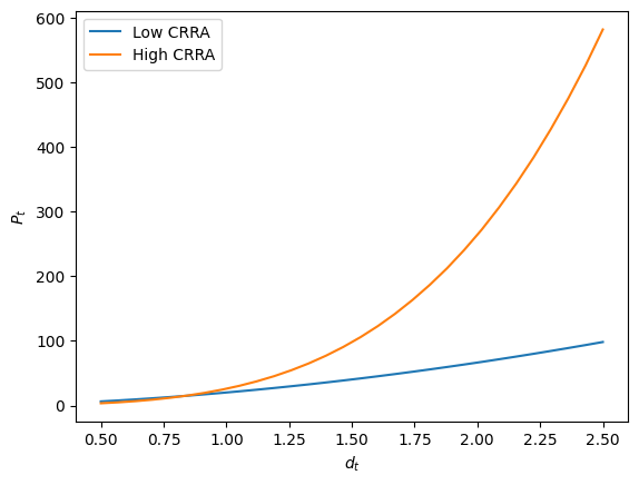

Testing our analytical solutions¶

Case 1: Log Utility¶

The lecture notes show that with logarithmic utility (a CRRA of 1), the pricing kernel has a closed form expression:

P^*(d_t) = \frac{d_t}{\vartheta}

(1)

We now compare our numerical solution with this analytical expression.

# Create an economy with log utility and the same dividend process from before
logUtilEcon = LucasEconomy(CRRA=1, DiscFac=Disc, DivProcess=DivProc)
# Solve it
logUtilEcon.solve()

# Generate a function with our analytical solution
theta = 1 / Disc - 1


def aSol(d):
    return d / theta


# Get a grid for d over which to compare them
dGrid = np.exp(DivProc.getLogdGrid())

# Plot both
plt.figure()
plt.plot(dGrid, aSol(dGrid), "*", label="Analytical solution")
plt.plot(dGrid, logUtilEcon.EqPfun(dGrid), label="Numerical solution")
plt.legend()
plt.xlabel("$d_t$")
plt.ylabel("$P^*(d_t)$")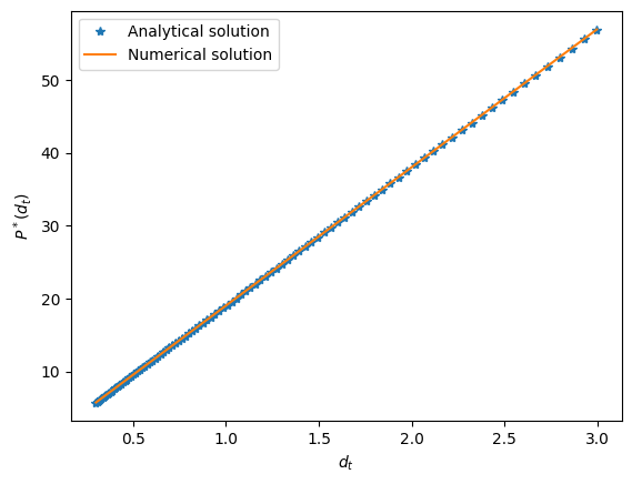

Case 2: I.I.D dividends¶

The notes also show that, if $\ln d_{t+n}\sim \mathcal{N}(-\sigma^2/2, \sigma^2)$ for all $n$ , the pricing kernel is exactly

P^*(d_t) = d_t^\rho\times e^{\rho(\rho-1)\sigma^2/2}\overbrace{\frac{\beta}{1-\beta}}^{=\vartheta}

We now our numerical solution for this case.

# Create an i.i.d. dividend process
σ = 0.1
iidDivs = DivProcess(α=0.0, σ=σ)

# And an economy that embeds it
CRRA = 2
Disc = 0.9

iidEcon = LucasEconomy(CRRA=CRRA, DiscFac=Disc, DivProcess=iidDivs)
iidEcon.solve()

# Generate a function with our analytical solution
dTil = np.exp((σ**2) / 2 * CRRA * (CRRA - 1))


def aSolIID(d):
    return d**CRRA * dTil * Disc / (1 - Disc)


# Get a grid for d over which to compare them
dGrid = np.exp(iidDivs.getLogdGrid())

# Plot both
plt.figure()
plt.plot(dGrid, aSolIID(dGrid), "*", label="Analytical solution")
plt.plot(dGrid, iidEcon.EqPfun(dGrid), label="Numerical solution")
plt.legend()
plt.xlabel("$d_t$")
plt.ylabel("$P^*(d_t)$")
plt.show()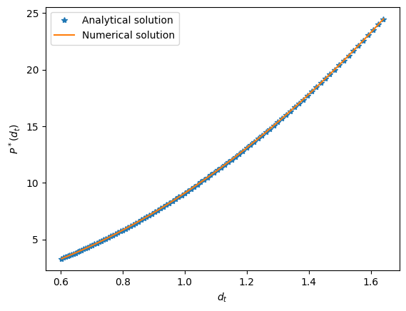

Case 3: Dividends that are a geometric random walk with drift¶

The notes also show that if the dividend process is

\ln d_{t+1} = \gamma + \ln d_t + \varepsilon_{t+1}, \qquad \varepsilon \sim \mathcal{N}(-\frac{\sigma^2}{2}, \sigma).

so that $E_t[d_{t+1}/d_t] = e^\gamma$ , then we have

P^*(d_t) = d_t^\rho\times e^{(\rho-1)\left(\rho\sigma^2/2 - \gamma\right)}\overbrace{\frac{\beta}{1-\beta}}^{\vartheta}

which, when $\rho=1$ , reduces (as it should) to

\frac{P^*(d_t)}{d_t} = \vartheta

CRRA = 2
Disc = 0.9
σ = 0.1
γ = 0.3

# Create a random walk dividend process
# (it turns out that the whole model can be normalized by d_t, and
# in normalized, terms the dividend proces becomes iid again)
rw_divs = DivProcess(γ=γ, α=0, σ=σ)

# And an economy that embeds it
rw_econ = LucasEconomy(CRRA=CRRA, DiscFac=Disc, DivProcess=rw_divs)
rw_econ.solve()

# Generate a function with our analytical solution
a_sol_factor = np.exp((CRRA - 1) * (CRRA * σ**2 / 2 - γ))


def a_sol_rw(d):
    return d**CRRA * a_sol_factor * Disc / (1 - Disc)


# Get a grid for d over which to compare them
dGrid = np.exp(rw_divs.getLogdGrid())

# Plot both
plt.figure()
plt.plot(dGrid, a_sol_rw(dGrid), "*", label="Analytical solution")
plt.plot(dGrid, rw_econ.EqPfun(dGrid), label="Numerical solution")
plt.legend()
plt.xlabel("$d_t$")
plt.ylabel("$P^*(d_t)$")
plt.show()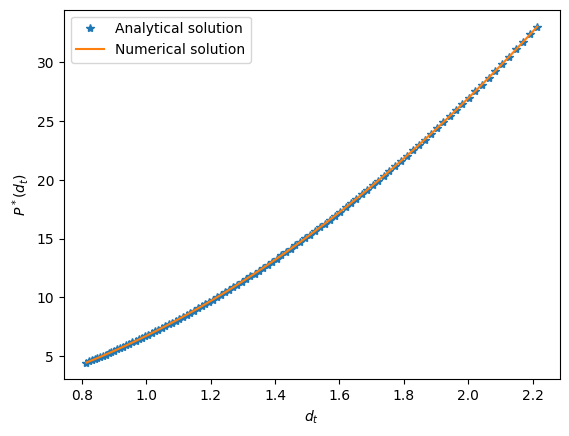

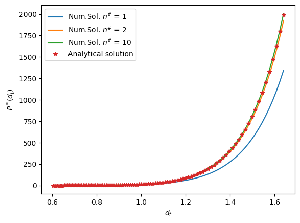
Testing our approximation of the dividend process¶

Hidden in the solution method implemented above is the fact that, in order to make expectations easy to compute, we discretize the random shock $\varepsilon_t$ , which is to say, we create a discrete variable $\tilde{\varepsilon}$ that approximates the behavior of $\varepsilon_t$ . This is done using a Gauss-Hermite quadrature.

A parameter for the numerical solution is the number of different values that we allow our discrete approximation $\tilde{\varepsilon}$ to take, $n^{\#}$ . We would expect a higher n^# to improve our solution, as the discrete approximation of $\varepsilon_t$ improves. We test this below.

# Increase CRRA to make the effect of uncertainty more evident.
CRRA = 10
Disc = 0.9
σ = 0.1
ns = [1, 2, 10]

dTil = np.exp((σ**2) / 2 * CRRA * (CRRA - 1.0))


def aSolIID(d):
    return d**CRRA * dTil * Disc / (1 - Disc)


dGrid = np.exp(iidDivs.getLogdGrid())

plt.figure()
for n in ns:
    iidDivs = DivProcess(α=0.0, σ=σ, nApprox=n)
    iidEcon = LucasEconomy(CRRA=CRRA, DiscFac=Disc, DivProcess=iidDivs)
    iidEcon.solve()
    plt.plot(dGrid, iidEcon.EqPfun(dGrid), label="Num.Sol. $n^\#$ = {}".format(n))

# Plot both
plt.plot(dGrid, aSolIID(dGrid), "*", label="Analytical solution")
plt.legend()
plt.xlabel("$d_t$")
plt.ylabel("$P^*(d_t)$")
plt.show()