The MPC out of Credit vs the MPC Out of Income

# Import the HARK ConsumerType we want
# Here, we bring in an agent making a consumption/savings decision every period, subject
# to transitory and permanent income shocks.
import matplotlib.pyplot as plt  # We need this module to change the y-axis on the graphs
from HARK.utilities import plot_funcs
from copy import deepcopy
from HARK.ConsumptionSaving.ConsIndShockModel import KinkedRconsumerType
from HARK.ConsumptionSaving.ConsIndShockModel import IndShockConsumerType

# Now, create an instance of the consumer type using the default parameter values
# We create the instance of the consumer type by calling IndShockConsumerType()
# We use the default parameter values by passing **Params.init_idiosyncratic_shocks as an argument
BaselineExample = IndShockConsumerType()

# Note: we've created an instance of a very standard consumer type, and many assumptions go
# into making this kind of consumer.  As with any structural model, these assumptions matter.
# For example, this consumer pays the same interest rate on
# debt as she earns on savings.  If instead we wanted to solve the problem of a consumer
# who pays a higher interest rate on debt than she earns on savings, this would be really easy,
# since this is a model that is also solved in HARK.  All we would have to do is import that model
# and instantiate an instance of that ConsumerType instead.  As a homework assignment, we leave it
# to you to uncomment the two lines of code below, and see how the results change!


BaselineExample = KinkedRconsumerType()

# Change the Default Riskfree Interest Rate
BaselineExample.Rfree = 1.02

# Change some parameter values
BaselineExample.Rfree = 1.02  # change the risk-free interest rate
BaselineExample.CRRA = 2.0  # change  the coefficient of relative risk aversion
BaselineExample.BoroCnstArt = -0.3  # change the artificial borrowing constraint
BaselineExample.DiscFac = (
    0.5  # chosen so that target debt-to-permanent-income_ratio is about .1
)
# i.e. BaselineExample.solution[0].cFunc(.9) ROUGHLY = 1.

# There is one more parameter value we need to change.  This one is more complicated than the rest.
# We could solve the problem for a consumer with an infinite horizon of periods that (ex-ante)
# are all identical.  We could also solve the problem for a consumer with a fininite lifecycle,
# or for a consumer who faces an infinite horizon of periods that cycle (e.g., a ski instructor
# facing an infinite series of winters, with lots of income, and summers, with very little income.)
# The way to differentiate is through the "cycles" attribute, which indicates how often the
# sequence of periods needs to be solved.  The default value is 1, for a consumer with a finite
# lifecycle that is only experienced 1 time.  A consumer who lived that life twice in a row, and
# then died, would have cycles = 2.  But neither is what we want.  Here, we need to set cycles = 0,
# to tell HARK that we are solving the model for an infinite horizon consumer.


# Note that another complication with the cycles attribute is that it does not come from
# Params.init_idiosyncratic_shocks.  Instead it is a keyword argument to the  __init__() method of
# IndShockConsumerType.
BaselineExample.cycles = 0

# Now, create another consumer to compare the BaselineExample to.

# The easiest way to begin creating the comparison example is to just copy the baseline example.
# We can change the parameters we want to change later.

XtraCreditExample = deepcopy(BaselineExample)

# Now, change whatever parameters we want.
# Here, we want to see what happens if we give the consumer access to more credit.
# Remember, parameters are stored as attributes of the consumer they are used for.
# So, to give the consumer more credit, we just need to relax their borrowing constraint a tiny bit.

# Declare how much we want to increase credit by
credit_change = 0.0001

# Now increase the consumer's credit limit.
# We do this by decreasing the artificial borrowing constraint.
XtraCreditExample.BoroCnstArt = BaselineExample.BoroCnstArt - credit_change

# First solve the baseline example.
BaselineExample.solve()

# Now solve the comparison example of the consumer with a bit more credit
XtraCreditExample.solve()

# First, declare useful functions to plot later


def FirstDiffMPC_Income(x):
    # Approximate the MPC out of income by giving the agent a tiny bit more income,
    # and plotting the proportion of the change that is reflected in increased consumption

    # First, declare how much we want to increase income by
    # Change income by the same amount we change credit, so that the two MPC
    # approximations are comparable
    income_change = credit_change

    # Now, calculate the approximate MPC out of income
    return (
        BaselineExample.solution[0].cFunc(x + income_change)
        - BaselineExample.solution[0].cFunc(x)
    ) / income_change


def FirstDiffMPC_Credit(x):
    # Approximate the MPC out of credit by plotting how much more of the increased credit the agent
    # with higher credit spends
    return (
        XtraCreditExample.solution[0].cFunc(x) - BaselineExample.solution[0].cFunc(x)
    ) / credit_change

# Now, plot the functions we want
%matplotlib inline
# Import a useful plotting function from HARK.utilities


# Declare the upper limit for the graph
x_max = 10.0


# Note that plot_funcs takes four arguments: (1) a list of the arguments to plot,
# (2) the lower bound for the plots, (3) the upper bound for the plots, and (4) keywords to pass
# to the legend for the plot.

# Plot the consumption functions to compare them
# The only difference is that the XtraCredit function has a credit limit that is looser
# by a tiny amount
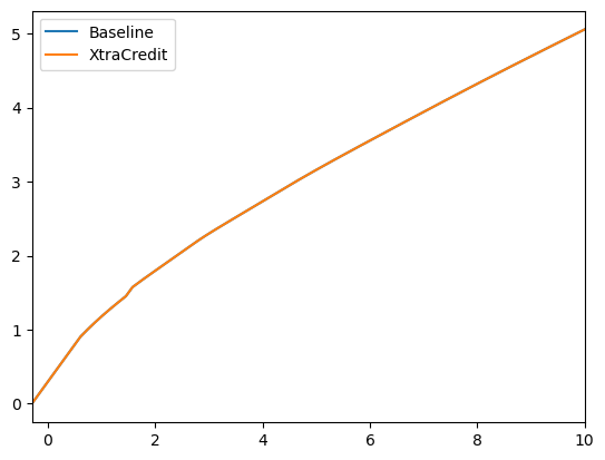
print(
    "The XtraCredit consumption function allows the consumer to spend a tiny bit more"
)
print(
    "The difference is so small that the baseline is obscured by the XtraCredit solution"
)
plot_funcs(
    [BaselineExample.solution[0].cFunc, XtraCreditExample.solution[0].cFunc],
    BaselineExample.solution[0].mNrmMin,
    x_max,
    legend_kwds={"loc": "upper left", "labels": ["Baseline", "XtraCredit"]},
)


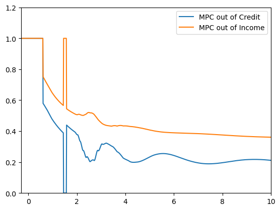
# Plot the MPCs to compare them
print("MPC out of Credit v MPC out of Income")
plt.ylim([0.0, 1.2])
plot_funcs(
    [FirstDiffMPC_Credit, FirstDiffMPC_Income],
    BaselineExample.solution[0].mNrmMin,
    x_max,
    legend_kwds={"labels": ["MPC out of Credit", "MPC out of Income"]},
)