 Powered by Econ-ARK
Generator: QuARK-make/notebooks_byname
Introduction
Buffer stock saving models of the kind implemented in say that, if a standard ‘Growth Impatience Condition’, holds:
then the ratio of asets to permanent income , , has a target value that depends on the consumer’s preferences (relative risk aversion , time preference ) and circumstances (interest factor , growth factor , uncertainty about permanent income shocks ).
If everyone had identical preferences and everyone were at their target , then inequality in the level of would be exactly the same as inequality in .
“The Distribution of Wealth and the Marginal Propensity to Consume” (Carroll, Slacalek, Tokuoka, and White 2017; hereafter: “cstwMPC”) shows that, when such a model is simulated and agents draw their idiosyncratic shocks (so, agents are ex post heterogeneous -- see the definition in Intro-To-HARK) -- asset inequality is indeed close to inequality even though everyone is not always at exactly their target .
But a large body of evidence shows that actual inequality in assets is much greater than actual inequality in permanent income. Thus, to make a model that qualifies as what cstwMPC call a ‘serious’ microfounded macro model of consumption (one that matches the key facts theory says should be first-order important), the model must be modified to incorporate some form of ex ante heterogeneity: That is, there must be differences across people in or or or or .
The most transparent and simplest of these to change is the time preference factor . So that is what the paper does. The main results are:
The distribution of need not be particularly wide to match the extreme concentration of wealth: roughly 0.91 to 0.98 (annual); that is, the most impatient person discounts the future about 6 percentage points more per year than the most patient agent agent
With such a distribution of , simulated agents’ (annual) marginal propensity to consume (MPC) from transitory income shocks to income matches large body of microeconomic evidence that typically finds evidence of MPC’s in the range of 0.2 to 0.6. This is much better than RA macro models that typically yield MPC’s in the range of 0.01 to 0.05.
While the most impatient agents in the cstwMPC model have fairly high MPCs (~0.6 annual), there is microeconomic evidence that a significant fraction of households have even higher MPCs than the model predicts, especially at the quarterly frequency. This group of households is commonly referred to as “hand-to-mouth” -- they consume most of their transitory shocks to income not too long after they receive them (mostly within a quarter). There are several reasons why a household could be hand-to-mouth, but one plausible explanation is that these households are even more impatient than estimated by cstwMPC for the most impatient agent.
# This cell does some setup and imports generic tools used to produce the figures

from HARK.utilities import get_lorenz_shares, get_percentiles
from HARK.Calibration import load_SCF_wealth_weights
from HARK.distributions import Uniform
from HARK.ConsumptionSaving.ConsIndShockModel import IndShockConsumerType
from copy import deepcopy
import warnings
from shutil import which
import matplotlib.pyplot as plt
from IPython import get_ipython  # In case it was run from python instead of ipython
from tqdm import tqdm

import numpy as np

Generator = False  # Is this notebook the master or is it generated?
# Import related generic python packages

# Set how many digits past the decimal point should be printed?


def mystr(number):
    return "{:.4f}".format(number)


def decfmt4(number):
    return "{:.4f}".format(number)


def decfmt3(number):
    return "{:.3f}".format(number)


def decfmt2(number):
    return "{:.2f}".format(number)


def decfmt1(number):
    return "{:.1f}".format(number)


# This is a jupytext paired notebook that autogenerates BufferStockTheory.py
# which can be executed from a terminal command line via "ipython BufferStockTheory.py"
# But a terminal does not permit inline figures, so we need to test jupyter vs terminal
# Google "how can I check if code is executed in the ipython notebook"


def in_ipynb():
    try:
        if (
            str(type(get_ipython()))
            == "<class 'ipykernel.zmqshell.ZMQInteractiveShell'>"
        ):
            return True
        else:
            return False
    except NameError:
        return False


# Determine whether to make the figures inline (for spyder or jupyter)
# vs whatever is the automatic setting that will apply if run from the terminal
if in_ipynb():
    # %matplotlib inline generates a syntax error when run from the shell
    # so do this instead
    get_ipython().run_line_magic("matplotlib", "inline")
else:
    get_ipython().run_line_magic("matplotlib", "auto")

# Import the plot-figure library matplotlib


# In order to use LaTeX to manage all text layout in our figures, we import rc settings from matplotlib.

plt.rc("font", family="serif")

# LaTeX is huge and takes forever to install on mybinder
# so if it is not installed then do not use it

iflatexExists = False
if which("latex"):
    iflatexExists = True

plt.rc("text", usetex=iflatexExists)

# The warnings package allows us to ignore some harmless but alarming warning messages

warnings.filterwarnings("ignore")
Calibrating a Basic Version of cstwMPC
To get started, let’s reproduce a simplified version of the main results from cstwMPC.
In cstwMPC, the authors calibrated nearly all of the model parameters-- risk aversion, income shock process, etc-- to commonly used or previously estimated values. The only parameter to be estimated is the distribution of . cstwMPC assumed that is uniformly distributed on , approximated by a seven point distribution.
Their estimation procedure seeks the values of and that generate a simulated distribution of wealth that best matches empirical U.S. data. Their definition of “best match” has two aspects:
The simulated aggregate capital-to-income ratio matches the true U.S. value.
The sum of squared distances between the simulated and empirical Lorenz curves (at the 20th, 40th, 60th, and 80th percentiles) is minimized (conditional on item 1).
cstwMPC’s target empirical moments are a capital-to-income ratio of 10.26 and cumulative wealth shares as given in the table below. Yes, you are reading the table correctly: The “poorest” 80 percent of households own 17.5 percent of wealth.
| Net worth percentile | Cumulative wealth share |
|---|---|
| 20th | -0.2% |
| 40th | 1.0% |
| 60th | 5.5% |
| 80th | 17.5% |
To reproduce their basic results, we must import an subclass and define a dictionary with calibrated parameters identical to those in the paper.
# Import IndShockConsumerType

# Define a dictionary with calibrated parameters
cstwMPC_calibrated_parameters = {
    "CRRA": 1.0,  # Coefficient of relative risk aversion
    "Rfree": [1.01 / (1.0 - 1.0 / 160.0)],  # Survival probability,
    # Permanent income growth factor (no perm growth),
    "PermGroFac": [1.000**0.25],
    "PermGroFacAgg": 1.0,
    "BoroCnstArt": 0.0,
    "CubicBool": False,
    "vFuncBool": False,
    "PermShkStd": [
        (0.01 * 4 / 11) ** 0.5
    ],  # Standard deviation of permanent shocks to income
    "PermShkCount": 5,  # Number of points in permanent income shock grid
    "TranShkStd": [
        (0.01 * 4) ** 0.5
    ],  # Standard deviation of transitory shocks to income,
    "TranShkCount": 5,  # Number of points in transitory income shock grid
    "UnempPrb": 0.07,  # Probability of unemployment while working
    "IncUnemp": 0.15,  # Unemployment benefit replacement rate
    "UnempPrbRet": 0.07,
    "IncUnempRet": 0.15,
    "aXtraMin": 0.00001,  # Minimum end-of-period assets in grid
    "aXtraMax": 40,  # Maximum end-of-period assets in grid
    "aXtraCount": 32,  # Number of points in assets grid
    "aXtraExtra": [None],
    "aXtraNestFac": 3,  # Number of times to 'exponentially nest' when constructing assets grid
    "LivPrb": [1.0 - 1.0 / 160.0],  # Survival probability
    "DiscFac": 0.97,  # Default intertemporal discount factor; dummy value, will be overwritten
    "cycles": 0,
    "T_cycle": 1,
    "T_retire": 0,
    # Number of periods to simulate (idiosyncratic shocks model, perpetual youth)
    "T_sim": 1200,
    "T_age": 400,
    "IndL": 10.0 / 9.0,  # Labor supply per individual (constant),
    "kLogInitMean": np.log(0.00001),
    "kLogInitStd": 0.0,
    "pLogInitMean": 0.0,
    "pLogInitStd": 0.0,
    "AgentCount": 10000,
}
Start with importing the predefined dictionaries for agent types from the HARK toolkit. Then only show the parameters that are actually different from the imported dictionary.
Creating an ex-ante distribution of heterogeneous agents
Now let’s make several instances of our class of agents and give them different values of , following cstwMPC’s estimated distribution. In our specification of interest, we will use and .
NB: Reported parameter estimates in cstwMPC use a model with aggregate shocks and wage and interest rates determined dynamically (a heterogeneous agents DSGE model); this is the in HARK. The estimated parameters are slightly different in this exercise, as we are ignoring general equilibrium aspects and only using the
Method 1: “Brute force” approach
There are two methods for accomplishing this. The first is a more “brute force” approach: We specify a uniform distribution and discretize it for the number of household types we would like to see in the model. From there, We place each of the household types with a different time preference factor in a list. Finally, a for-loop is used to compute the solution for each household’s optimization problem.
# This cell constructs seven instances of IndShockConsumerType with different discount factors

BaselineType = IndShockConsumerType(**cstwMPC_calibrated_parameters)

# Specify the distribution of the discount factor
num_types = 7  # number of types we want
DiscFac_mean = 0.9855583  # center of beta distribution
DiscFac_spread = 0.0085  # spread of beta distribution

# Here's how to use the tools to create time preference heterogeneity manually

DiscFac_dstn = (
    Uniform(DiscFac_mean - DiscFac_spread, DiscFac_mean + DiscFac_spread)
    .discretize(num_types)
    .atoms.flatten()
)

MyTypes = []  # initialize an empty list to hold our consumer types
for nn in range(num_types):
    # Now create the types, and append them to the list MyTypes
    NewType = deepcopy(BaselineType)
    NewType.DiscFac = DiscFac_dstn[nn]
    NewType.seed = nn  # give each consumer type a different RNG seed
    MyTypes.append(NewType)
Method 2: The new AgentPopulation class
The second approach incorporates a new class defined in the HARK toolkit: AgentPopulation. This class will create a new iterable object AgentPopulation, which takes two arguments. The first is the dictionary which defines the AgentType. The second is a distribution over the parameter value for which the user would like to see ex-ante heterogeneity in. From there, the approx_distributions method is called on the object to discretize the distribution given the specified number of discrete points. Finally, the create_distributed_agents method is called to create the distribution of agents, for which the standard solution method calls can be used to solve each agents problem.
# This cell constructs seven instances of IndShockConsumerType with different discount factors

from HARK.core import AgentPopulation

# Specify the distribution of the discount factor
num_types = 7  # number of types we want
DiscFac_mean = 0.9855583  # center of beta distribution
DiscFac_spread = 0.0085  # spread of beta distribution

cstwMPC_calibrated_parameters["DiscFac"] = Uniform(
    DiscFac_mean - DiscFac_spread, DiscFac_mean + DiscFac_spread
)

SubPops = AgentPopulation(IndShockConsumerType, cstwMPC_calibrated_parameters)
SubPops.approx_distributions({"DiscFac": {"N" : num_types}})
SubPops.create_distributed_agents()
Solving and Simulating the Baseline Agents
Now let’s solve and simulate each of our types of agents. If you look in the parameter dictionary (or at any of the agent objects themselves), you will see that each one has an attribute of 10000. That is, these seven ex ante heterogeneous types each represent ten thousand individual agents that will experience ex post heterogeneity when they draw different income (and mortality) shocks over time.
In the code block below, fill in the contents of the loop to solve and simulate each agent type for many periods. To do this, you should invoke the methods , , and in that order. Simulating for 1200 quarters (300 years) will approximate the long run distribution of wealth in the population.
After solving the model, we will check that the aggregate level of capital (total assets held by all households) to income ratio equals what we expected it would be. This will serve as a verification that the code is written correctly. To do this, we combine the asset holdings of all types, take the mean, and compare it to the desired capital to income ratio of 10.26.
NB: Because there is no permanent income growth in this model, all shocks are mean one and idiosyncratic, and we have many agents, aggregate or average income is 1.0.
1. Solution for the “brute force” approach
Here is the output for the solution to the first approach to the problem, as well as a computation of the mean level of assets across the agent types. As you can see, the model does a good job of matching the aggregate capital-to-output ratio found in the data, as cited by Carroll et al. (2017).
# Progress bar keeps track interactively of how many have been made
for ThisType in tqdm(MyTypes):
    ThisType.solve()
    ThisType.initialize_sim()
    ThisType.simulate()
100%|████████████████████████████████████████████████████████████████████████████████████| 7/7 [00:31<00:00, 4.46s/it]
aLvl_all = np.concatenate([ThisType.state_now["aLvl"] for ThisType in MyTypes])
print(
    "The ratio of aggregate capital to permanent income is "
    + decfmt2(np.mean(aLvl_all))
)
The ratio of aggregate capital to permanent income is 10.33
2. Solution using the AgentPopulation class
We now conduct the same exercise for the new tool implemented in HARK. As you can see, both the out for the solution and the mean level of assets are nearly identical to the output when using the “brute force” approach.
Note: As an aside, the working theory for why these two approaches give nearly-but-not-perfectly-identical solution outputs is that, the “brute force” approach requires the user to specify the random seed when creating the discretized distribution of agents. The approach using AgentPopulation, on the other hand, specifies the random seed for the user during the implementation of the code. As you may know from the basics of programming in Python, the random seed’s main function is for reproducibility of results when using random number generators. In order for this theory to be tested, the AgentPopulation tool in HARK must be updated to allow for users to fix the random seed in this way.
SubPops.solve()
SubPops.initialize_sim()
SubPops.simulate()

# time this second solution method
aLvl_all_ap = np.concatenate([ThisSubPop.state_now["aLvl"] for ThisSubPop in SubPops])
print(
"The ratio of aggregate capital to permanent income is "
+ decfmt2(np.mean(aLvl_all_ap))
)The ratio of aggregate capital to permanent income is 10.26
Plotting the Lorenz Curve
Next, we conduct the exercise of matching the inequality in the observable distribution of wealth using the distribution of assets that arises from the model we’ve constructed with ex-ante heterogeneity in the time preference factor. As you can see from the plots below, the matching exercise is again nearly identical from the two approaches.
# Compute Lorenz shares using the brute force approach

SCF_wealth, SCF_weights = load_SCF_wealth_weights()

pctiles = np.linspace(0.001, 0.999, 200)
sim_wealth = np.concatenate([ThisType.state_now["aLvl"] for ThisType in MyTypes])
SCF_Lorenz_points = get_lorenz_shares(
    SCF_wealth, weights=SCF_weights, percentiles=pctiles
)
sim_Lorenz_points = get_lorenz_shares(sim_wealth, percentiles=pctiles)

# Compute Lorenz shares using the `AgentPopulation` approach

sim_wealth_ap = np.concatenate([ThisSubPop.state_now["aLvl"] for ThisSubPop in SubPops])
SCF_Lorenz_points_ap = get_lorenz_shares(
    SCF_wealth, weights=SCF_weights, percentiles=pctiles
)
sim_Lorenz_points_ap = get_lorenz_shares(sim_wealth_ap, percentiles=pctiles)

# Plot Lorenz curves for model with uniform distribution of time preference using both methods

plt.subplot(1, 2, 1)
plt.plot(pctiles, SCF_Lorenz_points, "--k")
plt.plot(pctiles, sim_Lorenz_points, "-b")
plt.title("Brute force approach")
plt.xlabel("Percentile of net worth")
plt.ylabel("Cumulative share of wealth")

plt.subplot(1, 2, 2)
plt.plot(pctiles, SCF_Lorenz_points, "--k")
plt.plot(pctiles, sim_Lorenz_points_ap, "-b")
plt.title("Using AgentPopulation class")
# plt.xlabel("Percentile of net worth")
# plt.ylabel("Cumulative share of wealth")

plt.tight_layout()
plt.show(block=False)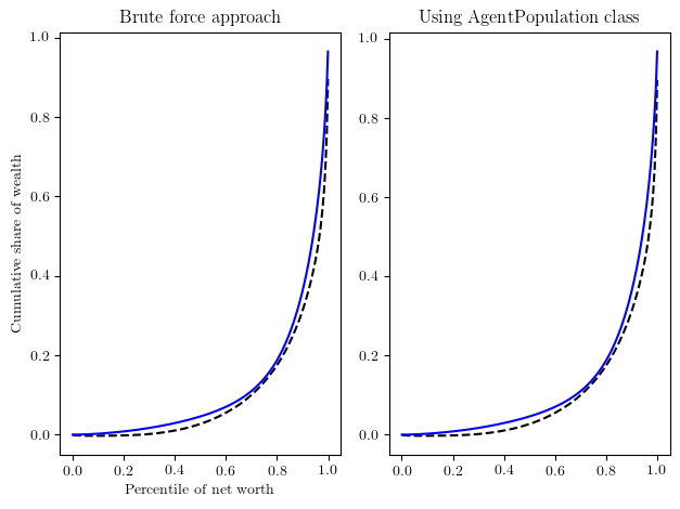
Calculating the Lorenz Distance at Targets
Now we want to construct a function that calculates the Euclidean distance between simulated and actual Lorenz curves at the four percentiles of interest: 20, 40, 60, and 80.
NB: For some reason, this step is not completed in the code. We leave this cell here, as this exercise should probably be performed as well.
The Distribution Of the Marginal Propensity to Consume
For many macroeconomic purposes, the distribution of the MPC is more important than the distribution of wealth. Ours is a quarterly model, and MPC’s are typically reported on an annual basis; we can compute a (very) approximate annual MPC from the quraterly ones as
In the cell below, we retrieve the MPCs from our simulated consumers and show that the 10th percentile in the MPC distribution is only about 6 percent, while at the 90th percentile it is almost 0.5
1. MPC distribution from the “brute force” approach
Again, we first show the computation from the “brute force approach”. This is done in the following code block.
# Retrieve the MPC's
percentiles = np.linspace(0.1, 0.9, 9)
MPC_sim = np.concatenate([ThisType.MPCnow for ThisType in MyTypes])
MPCpercentiles_quarterly = get_percentiles(MPC_sim, percentiles=percentiles)
MPCpercentiles_annual = 1.0 - (1.0 - MPCpercentiles_quarterly) ** 4

print(
    "The MPC at the 10th percentile of the distribution is "
    + str(decfmt2(MPCpercentiles_annual[0]))
)
print(
    "The MPC at the 50th percentile of the distribution is "
    + str(decfmt2(MPCpercentiles_annual[4]))
)
print(
    "The MPC at the 90th percentile of the distribution is "
    + str(decfmt2(MPCpercentiles_annual[-1]))
)
The MPC at the 10th percentile of the distribution is 0.06
The MPC at the 50th percentile of the distribution is 0.19
The MPC at the 90th percentile of the distribution is 0.51
2. MPC distribution from the AgentPopulation approach
Next, we compare this distribution of marginal propensities to consume with the one from the analogous computation when the AgentPopulation class is used. Notably, the distribution of MPCs in this case is nearly identical, with the only difference being at the 90th percentile.
# Retrieve the MPC's
percentiles = np.linspace(0.1, 0.9, 9)
MPC_sim_ap = np.concatenate([ThisSubPop.MPCnow for ThisSubPop in SubPops])
MPCpercentiles_quarterly_ap = get_percentiles(MPC_sim_ap, percentiles=percentiles)
MPCpercentiles_annual_ap = 1.0 - (1.0 - MPCpercentiles_quarterly_ap) ** 4

print(
    "The MPC at the 10th percentile of the distribution is "
    + str(decfmt2(MPCpercentiles_annual_ap[0]))
)
print(
    "The MPC at the 50th percentile of the distribution is "
    + str(decfmt2(MPCpercentiles_annual_ap[4]))
)
print(
    "The MPC at the 90th percentile of the distribution is "
    + str(decfmt2(MPCpercentiles_annual_ap[-1]))
)
The MPC at the 10th percentile of the distribution is 0.06
The MPC at the 50th percentile of the distribution is 0.19
The MPC at the 90th percentile of the distribution is 0.51
Adding Very Impatient Households
Now that we have some tools for examining both microeconomic (the MPC across the population) and macroeconomic (the distribution and overall level of wealth) outcomes from our model, we are all set to conduct our experiment.
In this exercise, we are going to add very impatient households to the economy in a very direct way: by replacing the most impatient consumer type with an even more impatient type. Specifically, we will have these agents have a discount factor of at a quarterly frequency, which corresponds to annual.
In the code block below, we:
Replicate the list of agents using .
Set the of the most impatient type to 0.80 (for the copied set of agents).
Solve and simulate the most impatient type (for the copied set of agents).
We conduct this exercise for both approaches again. The code is essentially identical, other than the naming conventions used for variables in each case. Notice that the output from each of the final two code blocks are exactly identical!
# Follow the instructions above to make another list of agents that includes *very* impatient households.
NewTypes = deepcopy(MyTypes)
NewTypes[0].DiscFac = 0.8
NewTypes[0].solve()
NewTypes[0].initialize_sim()
NewTypes[0].simulate()

# Retrieve the MPC's
percentiles = np.linspace(0.1, 0.9, 9)
MPC_sim = np.concatenate([ThisType.MPCnow for ThisType in NewTypes])
MPCpercentiles_quarterly = get_percentiles(MPC_sim, percentiles=percentiles)
MPCpercentiles_annual = 1.0 - (1.0 - MPCpercentiles_quarterly) ** 4

print(
    "The MPC at the 10th percentile of the distribution is "
    + str(decfmt2(MPCpercentiles_annual[0]))
)
print(
    "The MPC at the 50th percentile of the distribution is "
    + str(decfmt2(MPCpercentiles_annual[4]))
)
print(
    "The MPC at the 90th percentile of the distribution is "
    + str(decfmt2(MPCpercentiles_annual[-1]))
)

# these last two slides need an edit if this is the wealth distribution.
The MPC at the 10th percentile of the distribution is 0.06
The MPC at the 50th percentile of the distribution is 0.19
The MPC at the 90th percentile of the distribution is 0.97
# Follow the instructions above to make another list of agents that includes *very* impatient households.
NewSubPops = deepcopy(SubPops)
NewSubPops[0].DiscFac = 0.8
NewSubPops[0].solve()
NewSubPops[0].initialize_sim()
NewSubPops[0].simulate()

# Retrieve the MPC's
percentiles = np.linspace(0.1, 0.9, 9)
MPC_sim_ap = np.concatenate([ThisSubPop.MPCnow for ThisSubPop in NewSubPops])
MPCpercentiles_quarterly_ap = get_percentiles(MPC_sim_ap, percentiles=percentiles)
MPCpercentiles_annual_ap = 1.0 - (1.0 - MPCpercentiles_quarterly_ap) ** 4

print(
    "The MPC at the 10th percentile of the distribution is "
    + str(decfmt2(MPCpercentiles_annual_ap[0]))
)
print(
    "The MPC at the 50th percentile of the distribution is "
    + str(decfmt2(MPCpercentiles_annual_ap[4]))
)
print(
    "The MPC at the 90th percentile of the distribution is "
    + str(decfmt2(MPCpercentiles_annual_ap[-1]))
)
The MPC at the 10th percentile of the distribution is 0.06
The MPC at the 50th percentile of the distribution is 0.19
The MPC at the 90th percentile of the distribution is 0.97