Abstract
Korinek et al. (2026) publish three scenarios of AI’s effect on output, wages, and employment through 2030 and a browser explorer running their code. I reimplement the model as an Econ-ARK REMARK, with a script that fails whenever a number stops reproducing, and record twelve inputs, definitions, and orderings the paper leaves unstated. Every result they publish stands, from the scenarios’ paths to their robustness checks. With the twelve items, the reimplementation matches the explorer’s code to rounding error and every checkable published number. One more digit in the calibrated parameters recovers the few published results missed with them as printed. I plant mistakes in the code to compare the rounded published results and the explorer’s unrounded paths as reproducibility checks. Even a mistake too small to change a printed result moves the reimplementation’s paths away from the explorer’s. Checking a model therefore takes open code anyone can run, as REMARKs provide.
Key Points
The reimplementation matches the explorer’s monthly paths to within and all 226 checkable published numbers.
With the paper’s Table 1 parameters as printed, 163 of the 183 results reproduce; with one more digit, all 183.
Comparison with the tables detects four planted mistakes at 1 to 18 percent of full size; comparison with the explorer, at a billionth or less.
The largest mistake passing every table moves each published number at most 0.07 in printed units.
Introduction
How much could artificial intelligence change output, wages, and employment by 2030? Korinek et al. (2026) answer with three scenarios, modest, substantial, and extreme, computed from a monthly model of how the labor market adjusts as AI takes over tasks that people now do. In the extreme scenario GDP grows 15.4 percent a year and the unemployment rate of cognitive workers reaches 17.9 percent in 2030. The authors also publish the model as a scenario explorer at anthropic
Published models survive that treatment less often than one might hope. Given one textbook probit, five statistical packages declared convergence to five different answers McCullough & Vinod, 2003. In a journal archive that required authors to deposit their data and code, fewer than 15 of more than 150 empirical articles could be replicated McCullough et al., 2006. The replication files of 67 papers from 13 journals reproduce the key result of only about a third without the authors’ help, and of about half with it Chang & Li, 2022. Christensen & Miguel (2018) and Vilhuber (2020) survey that evidence and the practices that followed, from sharing data and code to journals checking reproducibility themselves. Against that record the paper stands out. Korinek et al. (2026) publish a research report outside any journal’s deposit policy, yet they print the model’s calibration and its full system of equations and publish code that runs it, which is what those replication attempts most often lacked.
With the paper and its code both public, a reader can ask a demanding question. Together, the paper and the explorer’s page print 226 numbers that a reader with public data can check, 43 inputs (the paper’s calibration) and 183 outputs that the model computes from them. If we write the model down from the paper’s description and feed it the printed inputs, do the printed outputs reproduce at the precision the paper prints them? That is a tall bar, probably one that few papers would clear. To find out, I reimplemented the model in plain Python from the paper’s Appendix A, the 44 equations of its Table A.1, and the calibration of its Table 1. Throughout, the reimplementation is that code, written from the paper’s description, and the reproduction its outcome, the paper’s numbers regenerated by that code.
Any description of a model in words leaves some details to its code. To reproduce the paper’s numbers exactly, I needed twelve items beyond its text. Some are inputs the paper prints rounded, some are definitions behind the numbers on the explorer’s page, and one is the order of two steps within a month. Fortunately, most of them can be read from the explorer’s code, since it holds the calibration at full precision (the “calibration record”) and the definitions behind its page’s numbers. For the rest, I choose the value or the order that makes the reproduction match the explorer’s monthly paths or a published number. Only the paper’s survey of US adults has no public source, since its microdata are confidential. Table 1 lists the twelve, with where each came from and what turns on it, and a test in the replication package checks each.
On their own, the printed inputs come close, since rounding an input shifts each output only slightly and a printed output changes only when it crosses a rounding boundary. Run on Table 1 exactly as printed, with the other eleven items in place, the model reproduces 163 of the 183 published outputs. Its 20 misses lie in Tables 3, 5, and 6, on the explorer’s page, and in Section 2.3.2’s normal-times steady state (the labor market before AI arrives, four of the 20); the 16 that belong to a scenario all lie in the substantial and extreme ones, none in the modest one. With every input printed to one more digit, all 183 reproduce. With all twelve items in place, the reproduction and the explorer’s code agree in every series and every month, with a largest gap of (the size of the rounding errors in the computer’s own arithmetic), across 25 cases, from the three scenarios to runs as long as 2040. All 226 checkable published numbers also reproduce within the paper’s printed rounding, so every result in its Tables 3, 5, and 6, in its text, and on the explorer’s page stands. The text and the tables differ in three small places, none of which moves a result, and of the thirteen calibration inputs that come from public data, eleven match their sources or come within a few percent while two remain open.
Only two of the twelve items move a published number in a way the paper’s own text and tables leave open. The first is Table 1’s precision, which accounts for all 20 misses (the calibration record holds, for example, the share of quits that responds to job prospects as 6/11, which Table 1 prints as 0.55). The second is an ambiguity in the equations. Each month some workers quit, and part of that quitting rises and falls with how easy it is to find a new job. The model converts each monthly quit fraction into a continuous rate, but the text does not say whether the conversion comes before or after quitting is split into its responsive part and the rest. Its wording reads more naturally as converting first. Matching the published tables alone cannot decide the order, since the responsive share they are read against is itself printed rounded. But at the explorer’s share of 6/11, only splitting first matches the tables. It alone also matches the explorer’s paths, which converting first misses by up to . I therefore split first.
A printed table is a coarse test of a reimplementation. Printed as 17.9, a number could be anything from 17.85 to 17.95, so a reimplementation can be wrong by a few hundredths and still match every table. To measure how coarse the tables are, I planted four mistakes in the code, each a plausible misreading of the paper, much as software testers seed deliberate faults (mutation testing, in their terms) to learn whether their tests catch them DeMillo et al., 1978, then shrank each mistake until a check missed it. Comparison with the explorer still detects all four when they are shrunk to between and 10-9 of full size. Comparison with the published tables, however, detects them only at 1 to 18 percent of full size, so for the tables each mistake must be 8.3 to 9.0 orders of magnitude larger. One more printed digit would narrow that range of 17.85 to 17.95 only tenfold.
Only the comparison with the explorer catches mistakes that small, so the package reruns it whenever the reimplementation’s code changes and fails whenever the comparison fails. This reproduction is an Econ-ARK REMARK (Reproductions and Explorations Made using ARK, the open-source Econ-ARK project behind the HARK toolkit for models of optimizing households Carroll et al., 2018), a public repository built around a script whose failure means the reproduction has failed. This report’s online supplement holds the model’s equations, every published number beside the reproduction’s value, the paper’s figures regenerated, the details of both checks, and a small version of the explorer whose cells run when the site is built.
The next section sets out the model and the explorer. What Reproduction Required, the heart of the report, takes up the twelve items, followed by notes on the paper’s text and its public data. The Checks and Detection Thresholds give the two checks and what each can detect. The package and a conclusion close the report.
The Model and Its Reimplementation
Section 2 and Appendix A of Korinek et al. (2026) are the model’s authoritative description. The supplement’s section on the model states every equation the reimplementation evaluates. This section gives only what a reader needs to follow the inventory and the checks.
AI enters through three scenario paths: the affected mass , the fraction of the economy’s tasks that AI can perform; the diffusion share , the fraction of those tasks’ instances performed with AI; and the log gain in productivity on each such instance. The first two follow logistic curves and the gain a straight line, the paper’s Equation (8),
where the affected mass rises toward the cognitive occupations’ share of the wage bill, which at the common wage is their share of employment, , and diffusion toward . All three scenarios share the mid-2026 anchors and and differ in their 2030 values, which fix the slopes and and the midpoints and . From at the base date , the gain’s line rises by a year. Each scenario also sets the automation share , the fraction of AI-performed instances that capital performs outright; the reinstatement ratio , the mass of new labor tasks created per unit of automated tasks; the search discount , which scales the job-finding chances of workers who look for work outside their old occupation group; and the speed at which firms post vacancies. Put plainly, a scenario states how much of the economy’s work AI can do, how much of that work is actually done with AI, how much more productive it is there, and how fast displaced workers find new jobs.
Given the rental rate of capital, a potential economy in which workers move freely between cognitive and all other occupations has a closed-form solution, the paper’s Proposition 1, for the labor share, the common wage, output per worker, and the capital stock, with tasks gross complements at an elasticity of substitution of 0.5 (so that output needs every task, and a task done slowly holds back the rest). Given a capital supply that rises with its return at an elasticity of 3, the reimplementation finds by bisection the rental rate that clears the capital market. That capital-supply schedule takes the place of saving, which the authors set aside deliberately. In their words the model “does not explicitly model” saving. With some capital possibly “financed from abroad,” their Footnote 5 notes, the split of output between consumption and investment need not be specified. Research input, a fixed fraction of GDP, raises the stock of labor-augmenting ideas through the paper’s Equation (42), in which more research speeds the growth of ideas while each further proportional gain gets harder to find as the stock grows (the “fishing-out” effect of semi-endogenous growth models). Through that stock, research feeds back into the wage and into measured TFP.
In the actual economy, by contrast, workers move between jobs only with time, and the model follows the two groups of workers through quits, layoffs, and matching. Part of normal quitting responds to job prospects, since workers quit more readily when new jobs are easy to find. A worker in group , cognitive or all other, quits at the rate
where is an exogenous base rate and scales the part that moves with the group’s job-finding rate last month, , relative to its normal value . On the model’s monthly grid, Appendix A converts every per-period fraction into a continuously compounded rate, so that a quit fraction enters as . Whether that conversion applies before or after the split into the two parts is the one ambiguity in the equations that moves a published number, taken up in What Reproduction Required. The cognitive wage adjusts gradually. The wage actually paid closes only part of its log gap each month to the wage that would clear the cognitive labor force attached to the group,
where is the common wage of the potential economy, the clearing wage, and the annual rigidity of the cognitive wage, 0.5 in every scenario, a real-wage rigidity of the kind studied by Blanchard & Galí (2007). The rigidity’s monthly weight on last month’s ratio is . At the sticky wage, firms demand fewer cognitive workers than are attached to the group (the employed plus the cognitive-origin unemployed above their normal pool), so quits from surplus positions go unreplaced and layoffs remove the rest. The unemployed search with the discount outside their group of origin, and hires follow the matching function of Haan et al. (2000), which turns each group’s searchers and job openings into hires. Each month the reimplementation solves the paper’s System (39), its conditions for output prices, both groups’ labor demands, and the capital market, three times: at the attached cognitive force, for the clearing wage; at the sticky wage, for cognitive labor demand; and at realized employment, for the actual economy’s GDP, all-other wage, rental rate, capital stock, and labor share. Before AI arrives, the normal-times steady state sets the unemployment pools, quit rates, vacancy-filling rates, and the efficiency of matching.
Beyond the monthly recursion of Appendix A, the reimplementation also covers the explorer’s alternative data sources and its quiz. It is about 1,300 lines of Python whose only dependency is numpy. One scenario runs to 2030 in a fraction of a second.
The explorer is the authors’ published code, a single JavaScript file (the bundle) served by anthropic.com and compressed for delivery, which shortens its variable names. Beyond the model’s code, the bundle holds two things the paper’s text does not: the calibration record behind Table 1, and the definitions behind the numbers on the explorer’s page (its dollar GDP, its split of workers, and its typical survey respondent). For the comparison of The Checks, the bundle’s model code is the reference solution, while its record and definitions are sources for Table 1. Because the authors publish the bundle without a license, the repository holds none of its code. Instead it holds a record of the bundle’s outputs, indexed by case and by a checksum (a fingerprint of the bundle’s exact contents), which the comparison reads.
The authors’ survey of US adults and its microdata, which are not public, underlie the paper’s Table 2, the columns of its Table 4 that describe US adults, its Figure 1, and the statement on the explorer’s page about the share of survey respondents. The reproduction covers everything else in the paper and on the explorer’s page, from public inputs.
What Reproduction Required
Table 1 lists the twelve items a reimplementation needs beyond the text, with where the paper stops on each, where each came from, and what turns on it. Most of them leave every published number where it is; I list them anyway, because a reader cannot know in advance which items matter. Recall that the two items below move published numbers in a way the paper’s own text and tables leave open.
The paper’s Table 1 prints its data inputs rounded, but the published tables come from the unrounded values in the explorer’s calibration record. The monthly job-loss rates, for example, are 0.8359 and 1.8379 percent in the two groups. Rounding them to 0.84 and 1.84 looks harmless; for most outputs it is. However, an output printed to one decimal changes its printed value whenever it crosses a rounding boundary, and a few outputs lie close to one. With the printed 0.84 and 1.84, the reproduction misses three published numbers. Run on all of that table’s printed shares, search pool, relative separation rates, and quit share, it misses 20 of the 183 published outputs, as the left panel of the supplement’s Figure S7 shows. One more printed digit in that table would let a reader reproduce the paper’s tables from the paper alone.
Appendix A converts quoted quit fractions into continuous rates, . I split each group’s normal quit fraction into the part that responds to job prospects, a share of 6/11 that the paper’s Table 1 prints as 0.55, and the rest, and then convert the month’s combined fraction. Converting before splitting, probably the more natural reading of Appendix A’s wording, moves the paths by up to and pushes 6 of the 226 published numbers out of their rounding. The six are four distinct values, since the extreme scenario’s average wage appears in three tables. The farthest, Table 6’s extreme all-other wage at , printed 70.1, becomes 70.0120, 0.088 from its printed value where rounding allows 0.05.
Matching the tables alone cannot tell the two orders apart, because a slightly different quit share offsets a change of order and Table 1 prints the share rounded, an offset the right panel of the supplement’s Figure S7 shows. Converting first reproduces all 226 published numbers at shares from 0.552 to 0.5545, which Table 1 would also print as 0.55, while splitting first needs shares from 0.5435 to 0.547. At exactly 0.55, the value Section 3.2 gives, neither order reproduces the tables. However, only splitting first reproduces them at 0.545, the share printed to one more digit. Fortunately, little depends on the choice. Converting first misses six published numbers at the explorer’s 6/11 and none at 0.553, inside its own window, and the two readings the tables accept differ by at most 0.011 in any published number. The second implementation of The Checks, written from the paper’s text alone, took the other reading.
Table 1:The inputs, definitions, and orderings a reimplementation needs beyond the paper’s text: where the text stops, where I took each from, and what turns on it.
| What the reproduction needed | Where the paper stops | Taken from | What turns on it |
| The paper’s Table 1 at full precision | prints them rounded | the explorer’s calibration record | 20 of 183 published outputs miss on the printed values |
| Quit fractions split into their two parts, then converted to rates | converts in Appendix A and splits in Equation (27); the order is unstated | the explorer’s paths | 6 published numbers miss the other way round |
| The responsive quit share, 6/11 | prints 0.55 | the explorer’s code | all 226 reproduce on 0.5435 to 0.5470, not at 0.55 itself |
| The log gain’s line, anchored at mid-2026 | writes Equation (8) from the 2024 base year | the paper’s Table 1 and the explorer | the 2030 gains of 0.300, 0.448, 0.800 |
| The ideas term in the wage | omits it in Equation (16), includes it in Table A.1 | Table A.1 | Section 2.1.3’s wage of 1.9 percent |
| Footnote 14’s posting speed and wage rigidity | states neither | matching: 0.25 and 0.5 | 3 fitted numbers |
| Footnote 14’s employment base | does not name it | matching: employment counted from mid-2026 | 84.25 on that base, 87.02 on the 2024 base |
| The page’s dollar scaling, worker split, and typical respondent | defines them only in the page’s code | the explorer’s code | 12 fitted numbers |
| Cognitive labor valued at its marginal product while the sticky wage is paid | leaves the difference implicit in System (39) | the explorer’s code | a profit of at most 0.31 percent of GDP |
| The bracket and the bisection counts | states neither | the explorer’s code: 100 halvings on [-4, 4], 200 for the steady state | nothing at the paper’s precision |
| The quiz’s ceilings on the gain and the slopes | states neither | the explorer’s code: ln 30 and 3 | nothing for the paper’s scenarios |
| The survey microdata | reports them in Table 2, Table 4, and Figure 1 | not public | those numbers and the page’s respondent share are excluded |
The supplement’s notes on the paper and its data detail four of these items, among them the two parameters of Footnote 14, which the footnote’s own numbers pin down.
Notes on the Paper and Its Data
Beyond the twelve items, two kinds of note remain, and both leave the results unchanged. In three passages the paper’s text and its tables differ, each probably for a simple reason. Thirteen of the calibration’s inputs come from public data, which the reproduction recomputes from the original sources.
Small Differences between the Text and the Tables
Section 4.2 describes the substantial scenario’s cognitive unemployment rate as rising “from 2.9 percent in mid-2026 to 4.5 percent in 2030, more than a 50 percent increase.” The reproduction gives 2.85 percent in 2024, 3.06 percent in mid-2026, and 4.53 percent in 2030, so the 4.5 percent in 2030 matches. The mid-2026 rate, which the explorer also gives, is above the 2024 one because Appendix A applies the scenario’s search discount from 2024, which raises unemployment a little before any displacement begins. Measured from mid-2026, the date the sentence gives, the rise in the cognitive unemployment rate is 48 percent, just under 50. However, the 2.9 percent is the 2024 rate, the normal-times steady state of Section 2.3.2, so the sentence probably measures from that starting level. On that base the rise in the rate is 59 percent, so the claim of more than 50 percent holds.
Section 2.1.3 illustrates the substantial scenario in 2030 with three numbers from the potential economy, a rental rate 4.6 percent above normal, a wage 1.9 percent above the path without AI, and an exact TFP gain of 0.029. The three do not come from one treatment of the stock of ideas: the wage of 1.9 percent includes the gain in that stock, while the TFP gain of 0.029 leaves it out. With or without the gain in that stock, the rental rate rounds to 4.6.
Footnote 14 reports that a transfer of 84 percent of the GDP gain would hold cognitive workers’ income at its level without AI. The reproduction recovers the 84 when it counts cognitive employment from mid-2026, the base Section 4.3 uses when it describes the extreme scenario’s cognitive jobs. With employment counted from 2024, the base of Table 3’s labor-income rows, the same transfer is 87 percent. The footnote’s number is presumably the mid-2026 figure. Its wording, however, which compares income with its level without AI, reads more naturally on the 2024 base.
Two points of notation remain, both rows of Table 1. Equation (8) writes the log gain as , with the base year set to 2024 in Table A.2, but the paper’s Table 1 gives the gain at the mid-2026 anchor. Table 1’s implied 2030 values of 0.30, 0.45, and 0.80 equal the anchor value plus three and a half years of slope, so the reproduction and the explorer start the line at mid-2026. Proposition 1’s wage, Equation (16), omits the ideas term that Table A.1’s wage row includes. I follow Table A.1, whose version also gives Section 2.1.3 its wage of 1.9 percent.
A date for the starting rate, a word on which channel each of those numbers includes, and the employment base behind the 84 would let a reader check each passage directly.
The Public Data behind the Calibration
For every input that comes from public data, the reproduction recomputes the value from its original source, in Table 2. Of the thirteen inputs, eleven match or are consistent and two remain open. “Matches” means the recomputation reproduces the printed value at its rounding. “Consistent” means the public source measures a close cousin of the paper’s statistic, such as seasonally adjusted gross flows in place of matched IPUMS records (respondents linked across months), and falls within a few percent of the printed value or inside its printed range. “Open” means I have not pinned down why the recomputation departs from the printed value: observed exposure, the measure behind the affected mass’s mid-2026 anchor of 0.14, falls more than a tenth short of its printed value for cognitive work and overall; the standard specification of the quits elasticity gives 0.54 where two monthly variants round to the printed 0.53. The paper’s job-finding and separation statistics come from matched IPUMS-CPS records, which require an account to download. BLS data and the replication files of Carrillo-Tudela & Visschers (2023) give public cross-checks that fall within a few percent.
Table 2:The calibration’s public inputs recomputed from their original sources.
| Input | Paper | Public recomputation | Source | Status |
|---|---|---|---|---|
| Cognitive share of employment | 0.624 | 0.6235 | CPS 2025 annual averages, BLS Table 11 | matches |
| Normal search pool, share of the labor force | 0.038 | 0.0384 | CPS 2025 annual averages, BLS Tables 11 and 25 | matches |
| Vacancy filling | 4.0 percent a working day, 26 days, 0.65 within a month | 3.987 percent, 25.92 days, 0.6528 | JOLTS, following Davis et al. (2013) | matches |
| Firm use of AI | 18 percent of firms, 32 employment-weighted; 23 with worker task use | the same | Bonney et al. (2026) | matches |
| Automation share of AI use | about half on Claude.ai, three quarters on the API | the same | Appel et al. (2025) | matches |
| Rated feasibility of cognitive work | 2030 affected mass between 0.2 and 0.5 | 0.4334, employment-weighted | Eloundou et al. (2024) | consistent |
| Job finding from unemployment, per month | 0.219 | 0.2243 | BLS gross flows, 2010-19 | consistent |
| Job loss from employment, per month | 1.22 percent | 1.2547 percent | BLS gross flows, 2010-19 | consistent |
| Separation rate, other relative to cognitive | 2.20 | 2.0968 | BLS short-term unemployment by last occupation, 2011-19 | consistent |
| Job finders changing group: from cognitive, from other, all | 18.7, 11.2, 14.3 percent | 18.31, 11.32, 14.26 percent | Carrillo-Tudela & Visschers (2023), IPUMS-CPS excerpt, 2010-19 | consistent |
| Normal search discount | 0.17 | 0.1692 | from the switching shares above | consistent |
| Elasticity of quits to job finding | 0.53 | 0.5279 and 0.5286 in two monthly specifications, 0.5379 in the standard one | JOLTS quits and CPS flows, 2001-19 | open |
| Observed exposure, mid-2026: cognitive, other, overall | 0.22, 0.01, 0.14 | 0.1888, 0.0097, 0.1212 | Massenkoff & McCrory (2026), CPS weights | open |
For observed exposure, the gap between the recomputation and the paper probably comes from how occupation-level scores are aggregated onto the CPS’s occupation lines. Where one line combines several detailed occupations, I average them without weights, since no sub-weights are published. The code for every row is in code/validation/upstream_*.py.
The Checks
The first check compares the reproduction with the explorer’s own code in every series the explorer reports and every month. A validation script downloaded the explorer’s code from the authors’ site, confirmed from its checksum that it was the recorded version, and ran its model code with the same scenario and calibration as the reproduction, once for every case the comparison uses; the test suite replays that record. In the left panel of Figure 1 we plot the largest gap in each of 25 cases: the three scenarios; the robustness settings of Tables 5 and 6; the linearized model, in which the first-order rows of Table A.1 replace the exact ones; two points away from the calibration, run to 2032 and 2035; seven sets of answers to the explorer’s quiz; its five data options; and two runs to 2040. At its widest, the gap of lies far inside a tolerance of 10-12, which I set well above the rounding error a computer accumulates on numbers of order one over 72 to 192 monthly steps, in each of which the reimplementation runs four bisections of 100 halvings, one for the potential economy’s rental rate and three for System (39). Up to the computer’s own rounding, then, the two programs compute the same numbers.
Next, we compare the published numbers with the reproduction. We count a number as reproduced when the reproduction’s value rounds to it at the precision the paper prints. Of the 226 published numbers, 211 are “predicted,” in the sense that the paper’s text states how each is computed before any comparison, so matching one tests the reproduction. Another 15 are “fitted,” in the sense that I took a definition or an unstated parameter from the explorer or chose it by matching, which makes matching them a weaker test. Split the other way, 43 are inputs the model takes as given, which no error in its dynamics could move, and 183 are outputs the simulation produces. Table 3 counts them by source. The right panel of Figure 1 shows all 226 inside their rounding.
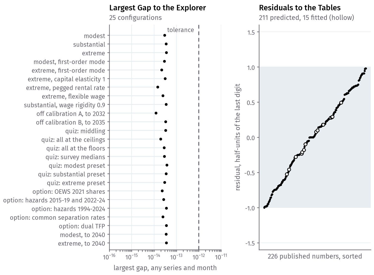
Figure 1:Left: the largest gap between the reproduction and the explorer, over every series and every month, for each of 25 cases. Right: each of the 226 published numbers’ gap to its printed value, scaled so that 1 marks the edge of its rounding, with the printed rounding shaded.
Table 3:Every number the paper and the explorer’s page print that can be reproduced from public inputs, by source, split into predicted and fitted numbers and into inputs and outputs as the text defines them. The last column counts the numbers reproduced at the paper’s rounding.
| Source | Predicted | Fitted | Inputs | Outputs | Within rounding |
| Table 3 | 60 | 0 | 0 | 60 | 60 of 60 |
| Table 5 | 40 | 0 | 0 | 40 | 40 of 40 |
| Table 6 | 49 | 0 | 0 | 49 | 49 of 49 |
| Footnote 14 | 0 | 3 | 0 | 3 | 3 of 3 |
| Section 2.3.2 | 11 | 0 | 0 | 11 | 11 of 11 |
| Table 1 | 5 | 0 | 5 | 0 | 5 of 5 |
| Table A.2 | 6 | 0 | 6 | 0 | 6 of 6 |
| Section 2.1.3 | 3 | 0 | 0 | 3 | 3 of 3 |
| Section 4.2 | 1 | 0 | 0 | 1 | 1 of 1 |
| Section 2.2.1 | 1 | 0 | 0 | 1 | 1 of 1 |
| Section 4.3 | 1 | 0 | 0 | 1 | 1 of 1 |
| Table B.1 | 30 | 0 | 30 | 0 | 30 of 30 |
| Appendix B.3 | 1 | 0 | 1 | 0 | 1 of 1 |
| Section 3.2 | 1 | 0 | 1 | 0 | 1 of 1 |
| Explorer page | 2 | 12 | 0 | 14 | 14 of 14 |
| All | 211 | 15 | 43 | 183 | 226 of 226 |
Comparison with a published number detects a mistake only when the mistake pushes that number across a rounding boundary, so what the second check can detect depends on the numbers that lie closest to their boundaries. Cognitive unemployment in the extreme scenario, 17.94905 in the reproduction and printed as 17.9, lies only 0.00095 below its rounding boundary at 17.95. The supplement’s Figure S6 shows every output’s margin.
Beside the two checks, a third comparison tests how the text is read. Claude Code (Anthropic’s coding agent), running Opus 5 and restricted to the paper’s text, wrote a second implementation of the model with the explorer’s code and this reproduction’s code withheld from it. Once the restriction was lifted, I verified that the second implementation uses only the paper’s printed inputs. The second implementation is independent of the explorer and of this reproduction, though not of this report’s author. Its own list of targets, transcribed by hand from the paper and separate from the 226 published numbers here, happens also to hold 211. Under the best readings of the text it could find, the second implementation reproduces 199 of them. Its misses trace to the printed calibration it runs on, to the quit order, and to the mid-2026 rate the notes take up. On the quit order it converts before splitting. Appendix A says the rows of Table A.1 hold exactly given their right-hand sides. The quit row holds that way, in the rate actually applied, only when quits are converted first, which probably makes converting first the more natural reading of the text alone. Given the same data inputs as this reproduction, the second implementation’s monthly paths come within to of this reproduction’s, depending on the case, and the whole gap comes from the quit order. Indeed, with that order aligned, the two implementations agree to . The comparison covers the model’s monthly paths. It leaves out how numbers are reported, Footnote 14, and the explorer’s page.
Detection Thresholds
To measure what each check can reject, I plant four mistakes in the reimplementation’s own code. Each is a misreading of the paper that a careful reader could plausibly make, with only a modest effect on the 2030 aggregates:
quits enter the equations for worker flows as the quoted monthly fraction, never converted to the continuous rate of Appendix A;
those equations aim at this month’s targets instead of next month’s, a one-month timing error;
the paper’s first-order approximations (the first-order rows of Table A.1) replace its exact equations;
the normal-times steady state is solved at the scenario’s search discount instead of the normal-times one.
At full strength both checks detect each of the four planted mistakes. The largest gaps to the explorer range from to . Entering quits unconverted produces the smallest gap and moves only 8 published numbers outside their rounding, because at the normal monthly quit fractions of 0.6 and 1.4 percent a fraction and its continuous rate differ by less than one percent of the fraction. Each of the other three changes the worker flows or the potential economy directly and moves 65 to 72 published numbers.
How weak a mistake can each check still detect? The strength of a planted mistake can be thought of as a dial: at 1 the mistake is fully present, at 0 it is gone, and in between each planted quantity is times its correct value plus times the erroneous one. We turn the dial down over twelve orders of magnitude and record, for each check, the weakest version of each mistake it still detects.
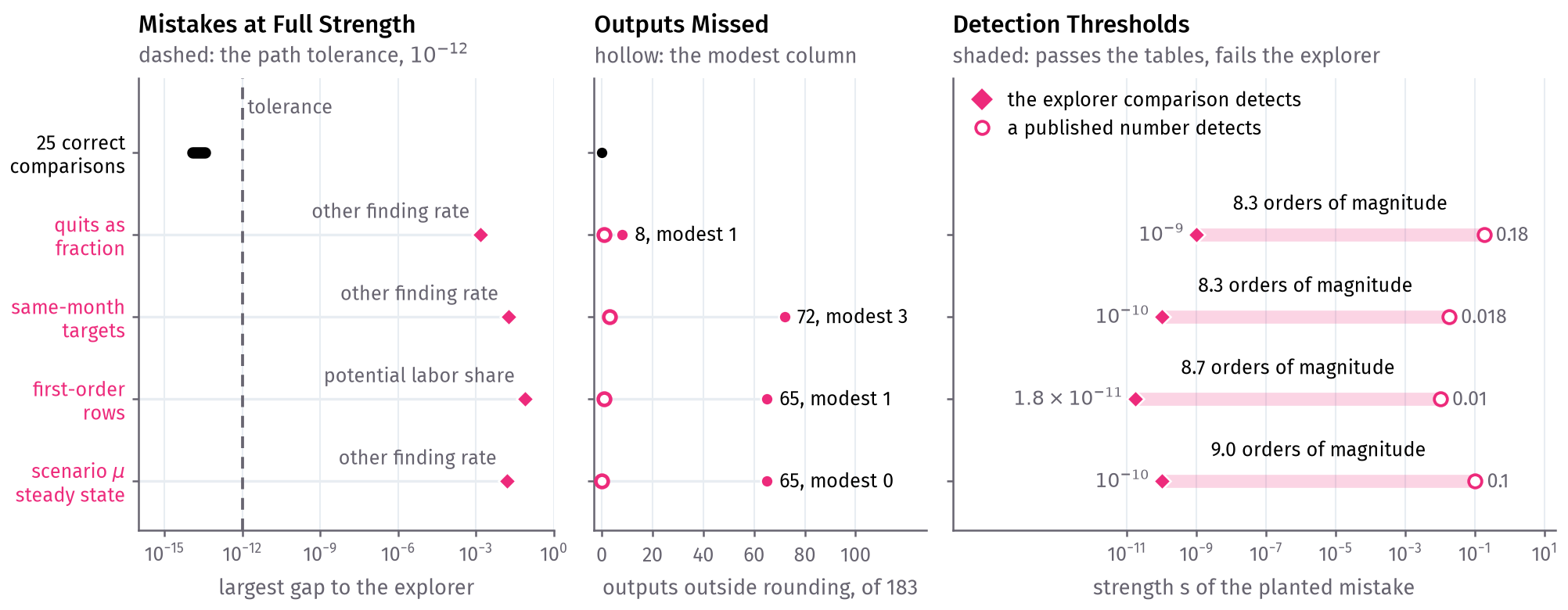
Figure 2:Left: the full-strength gaps, labeled with the series where each is largest, against the 25 correct comparisons. Middle: published outputs outside their rounding at full strength, over all outputs and over the modest scenario’s column alone. Right: for each planted mistake, in the same row order, the span of strengths that passes all 226 published numbers and still fails the explorer comparison.
Against the explorer, the four planted mistakes are detected from strengths between and 10-9. That threshold is simply the 10-12 tolerance on the monthly paths divided by the mistake’s full-strength gap, rounded up to the dial’s grid of four strengths per factor of ten, evenly spaced in logs, because a weak mistake’s gap grows in proportion to its strength. By contrast, comparison with the published numbers detects the mistakes only from strengths between 0.01 and 0.18, for each mistake 8.3 to 9.0 orders of magnitude above the explorer’s threshold. It follows that a planted mistake can shift the monthly paths by as much as a thousandth and still leave every published number inside its rounding.
The tables’ thresholds come from a few numbers. For three of the four planted mistakes, the first number to fail is the extreme scenario’s cognitive unemployment, which lies just below its rounding boundary. The fourth mistake, the steady state solved at the scenario’s search discount, first moves extreme GDP growth (15.445 percent a year, printed 15.4) and the substantial scenario’s wage in all other occupations (5.863 percent above its path without AI, printed 5.9), which responds strongly to the search discount. At full strength about two thirds of the rejections come from the extreme scenario’s columns, while the modest scenario’s column loses between none and three published numbers per mistake. Each mistake distorts how the economy adjusts to AI and so matters more the further a scenario moves the economy. The modest scenario’s search discount equals the normal-times one, so the fourth mistake leaves the modest scenario’s paths unchanged. Under each of the other three, the median published output of the extreme scenario moves about forty times as far as the modest scenario’s.
But the mistakes that pass the tables are small. The strongest version of each mistake that still passes all 226 published numbers changes each of them by at most 0.07 in the units the paper prints, against 0.13 to 2.5 at full strength. For these four mistakes, then, a reimplementation that agrees with the published tables differs from the authors’ model by economically negligible amounts.
The Package
An Econ-ARK REMARK is a public repository, indexed in the Econ-ARK catalog, whose standard has one operative rule: the package’s script must reproduce every result its authors claim. In the standard’s words, “if this script fails, your reproduction is assumed to not have worked.” Around that script, reproduce.sh, the standard requires a recipe for a fixed software environment (a Dockerfile), a README, a license, a tagged release, and, at its highest tier, a Zenodo DOI (a permanent identifier for an archived snapshot) bound to one version of the code. I chose to have the script check everything the report says.
Running the script builds that environment, downloads the public data behind the calibration recheck from their original sources, runs the test suite, and builds the site. Its test suite requires the tables of the report and the supplement, Table 1 included, to equal what the reimplementation computes now, and each of the 226 published numbers to print as published at its rounding. It also replays the explorer’s recorded outputs against the reproduction in every series and every month, runs the four planted mistakes at full strength and at their thresholds, and recomputes the calibration’s public inputs from their sources, where a missing source file fails the suite. Because the site build executes the supplement’s cells, the supplement’s tables are outputs of the same code. In addition, the package holds the second implementation, with the test that compares the two and isolates the quit order as their only difference.
This report’s strongest check depends on the authors’ explorer, which the script runs in a fixed environment against one recorded version of the explorer’s code. Most of the twelve items appear in no printed source: the calibration record and the definitions behind the page’s numbers, for example, are in the explorer’s code, and Footnote 14’s parameters follow from the footnote’s own numbers by matching. The package supplies each of them and keeps them under test. Stated in a document, they would hold only until either program changed. The script, however, fails whenever a change to the reimplementation’s code moves a published number or a recorded path. If the authors redeploy the explorer, its code no longer matches the recorded checksum, so the script that refreshes the record stops and reports the redeployment.
Conclusion
The results of Korinek et al. (2026) stand: the three scenarios’ paths for output, wages, employment, and capital through 2030, and their reruns at other elasticities of capital supply and other rigidities of the cognitive wage. Because the authors publish their calibration, their equations, and code that runs the model, their model can be reimplemented from their Appendix A once the twelve items of Table 1 are in hand, most of them from the explorer’s code. With those items the reimplementation matches the explorer’s own code to within and all 226 checkable published numbers within their rounding. As for any paper, matching the tables establishes less than matching the explorer, since a mistake that shifts the monthly paths by as much as a thousandth can leave every printed number unchanged, and the tables leave open the one ambiguity in the model’s equations that moves a published number. Nine of the twelve items would be easy additions to a later version of the paper, a sentence each, one of them only a single extra printed digit in its Table 1. Three belong elsewhere: the definitions on the explorer’s page, its quiz bounds, and the confidential survey. Even if a later version stated all nine, only a script would keep them true.
This report also answers a question the paper’s own robustness checks leave aside. In its Tables 5 and 6 the paper varies the elasticity of capital supply and the rigidity of the cognitive wage, while I vary how the text is read. It turns out that the results hardly depend on the reading. Between the two readings of the quit equation that the tables accept, each published number differs by at most 0.011. Likewise, the planted mistakes that pass the tables change each published number by at most 0.07.
Of course, a reproduction confirms the arithmetic that carries the scenarios’ assumptions to their results, and none of the assumptions themselves. The pace at which AI reaches the economy’s tasks, the paths of (1), is one of them. Jones & Tonetti (2026) argue that growth accelerates far more slowly than automation spreads, because when tasks are weak links, output is held back by the tasks that slowly improving labor still performs. The scenarios’ model shares those weak links, since its tasks are gross complements, so in the scenarios the pace comes from the assumed paths.
Econ-ARK will use this reproduction to develop models in which household saving, which the authors set aside deliberately, supplies the economy’s capital. In those models the capital stock becomes an outcome of the scenario, whose distributional effects can then be measured household by household. The monthly transitions recovered here, which neither the paper nor the explorer displays, are the income risk those households would face.
This reproduction is independent work, done in good faith and out of admiration for the original. It is not an Anthropic product. Neither Anthropic nor the paper’s authors have reviewed or endorsed it. The model and its ideas belong to the authors; any mistake in the reproduction is mine.
During the preparation of this work the author used Claude Code (Anthropic) to assist in editing and revising the prose and the code, and in checking the numerical claims in the text against the reproduction’s code. The second implementation of The Checks is the tool’s own work: Claude Code wrote it from the paper’s text alone, with the explorer’s code and the reproduction’s code withheld, and the author then verified that it uses only the paper’s printed inputs. After using this tool, the author reviewed and edited the content as needed and takes full responsibility for the content of the publication.
Acknowledgments
I thank the authors for a paper detailed enough to reimplement and for an explorer that makes every scenario easy to see, and Christopher Carroll for comments on this report and on the household work that builds on it.
Data Availability
The reproduction’s code and tests are in its replication package, under code/econ_scenarios/ and code/validation/. Because the explorer is published without a license, the package holds a record of the explorer’s outputs and none of its code, with the script that downloads the authors’ bundle and regenerates the record. The scripts code/validation/upstream_*.py download the public data behind the recheck of the calibration from their original sources. The matched IPUMS-CPS records require an account.
- Korinek, A., Jones, C. I., Sacher, S., Cotter, T., & McCrory, P. (2026). Economic Scenarios for Transformative AI [Working Paper 2026-02]. The Anthropic Institute. https://www.anthropic.com/institute/econ-scenarios
- McCullough, B. D., & Vinod, H. D. (2003). Verifying the Solution from a Nonlinear Solver: A Case Study. American Economic Review, 93(3), 873–892. 10.1257/000282803322157133
- McCullough, B. D., McGeary, K. A., & Harrison, T. D. (2006). Lessons from the JMCB Archive. Journal of Money, Credit, and Banking, 38(4), 1093–1107. 10.1353/mcb.2006.0061
- Chang, A. C., & Li, P. (2022). Is Economics Research Replicable? Sixty Published Papers from Thirteen Journals Say “Often Not.” Critical Finance Review, 11(1), 185–206. 10.1561/104.00000053
- Christensen, G., & Miguel, E. (2018). Transparency, Reproducibility, and the Credibility of Economics Research. Journal of Economic Literature, 56(3), 920–980. 10.1257/jel.20171350
- Vilhuber, L. (2020). Reproducibility and Replicability in Economics. Harvard Data Science Review, 2(4). 10.1162/99608f92.4f6b9e67
- DeMillo, R. A., Lipton, R. J., & Sayward, F. G. (1978). Hints on Test Data Selection: Help for the Practicing Programmer. Computer, 11(4), 34–41. 10.1109/C-M.1978.218136
- Carroll, C., Kaufman, A., Kazil, J., Palmer, N., & White, M. (2018). The Econ-ARK and HARK: Open Source Tools for Computational Economics. Proceedings of the 17th Python in Science Conference, 25–30. 10.25080/majora-4af1f417-004
- Blanchard, O. J., & Galí, J. (2007). Real Wage Rigidities and the New Keynesian Model. Journal of Money, Credit and Banking, 39(s1), 35–65. 10.1111/j.1538-4616.2007.00015.x
- den Haan, W. J., Ramey, G., & Watson, J. (2000). Job Destruction and Propagation of Shocks. American Economic Review, 90(3), 482–498. 10.1257/aer.90.3.482
- Carrillo-Tudela, C., & Visschers, L. (2023). Unemployment and Endogenous Reallocation over the Business Cycle. Econometrica, 91(3), 1119–1153. 10.3982/ECTA12498
- Davis, S. J., Faberman, R. J., & Haltiwanger, J. C. (2013). The Establishment-Level Behavior of Vacancies and Hiring. Quarterly Journal of Economics, 128(2), 581–622. 10.1093/qje/qjt002
- Bonney, K., Breaux, C., Dinlersoz, E., Foster, L., Haltiwanger, J., & Pande, A. (2026). The Microstructure of AI Diffusion: Evidence from Firms, Business Functions, and Worker Tasks (Working Paper CES-WP-26-25). U.S. Census Bureau, Center for Economic Studies.
- Appel, R., McCrory, P., Tamkin, A., Stern, M., McCain, M., & Neylon, T. (2025). Anthropic Economic Index Report: Uneven Geographic and Enterprise AI Adoption [Report]. Anthropic.
- Eloundou, T., Manning, S., Mishkin, P., & Rock, D. (2024). GPTs are GPTs: Labor Market Impact Potential of LLMs. Science, 384(6702), 1306–1308. 10.1126/science.adj0998