Supplement to Reproducing “Economic Scenarios for Transformative AI”
This supplement to Reproducing “Economic Scenarios for Transformative AI” holds the model’s equations with the module that evaluates each, every published number beside the reproduction’s value, the paper’s figures regenerated from the reproduction, the details of the two checks, the remaining notes on the paper and its data, and a small version of the authors’ explorer, the web page that runs their model in the reader’s browser. The supplement’s code cells are executable.
Running the Code
Every output on this page was computed when the site was built, from the same files that the test suite runs. To run the cells yourself, build the page locally:
uv sync
uv run pytest
uv run myst build --html --execute
From code/, the command uv run python -m validation.gate runs both checks and every test with a “planted mistake”, in the sense of a plausible misreading of the paper put into the reimplementation’s code on purpose to see whether the checks catch it. Refreshing the stored record of the explorer’s outputs after the authors update their page needs Node.js (a JavaScript runtime that works outside a browser), as code/validation/oracle.py describes. The second implementation of the report’s third comparison, written from the paper’s text alone, is code/cleanroom, and code/validation/cleanroom.py compares it with the reimplementation path by path. It turns out that the two differ only in the order in which quit fractions are split and converted to rates (The Model in Brief), as the tests in code/tests/test_cleanroom.py show.
Source
# Make the repository's code importable. A local build runs this page in a Jupyter kernel beside
# the repository. The emscripten branch below is for a kernel in the reader's browser, which this
# website cannot yet start (see Interactive Scenarios); such a kernel would read the same files
# from this website and install ipywidgets for the sliders.
import importlib.util
import logging
import sys
from pathlib import Path

try:
    from pyodide.http import open_url  # the browser kernel only
except ImportError:
    open_url = None

# The browser kernel builds matplotlib's font cache on first import, with a notice; keep it quiet.
font_log = logging.getLogger("matplotlib.font_manager")
font_log.setLevel(logging.ERROR)
import matplotlib.pyplot as plt  # imported here so that the browser kernel loads the package
import numpy as np

font_log.setLevel(logging.NOTSET)

if sys.platform == "emscripten":
    kernel = importlib.util.module_from_spec(importlib.util.spec_from_loader("kernel", loader=None))
    sys.modules["kernel"] = kernel
    exec(open_url("kernel.py").read(), kernel.__dict__)

    await kernel.prepare(widgets=True)
else:
    root = next(p for p in (Path.cwd(), *Path.cwd().parents) if (p / "code" / "econ_scenarios").is_dir())
    sys.path.insert(0, str(root / "code"))
The Model in Brief
Section 2 and Appendix A of Korinek et al. (2026) are the authoritative description of the model. This supplement follows their symbols and their equation numbers; each part below gives the module of the code that computes it.
Scenarios
AI enters the model through how large a share of tasks it can perform, how widely it spreads, how much it raises output where it is used, and how much it disrupts workers. In their Table 1, Korinek et al. (2026) set these for three scenarios; the table below prints them as the code stores them.
import pages

pages.scenario_table()The paper’s Equation (8) gives the paths of the first three over the date , in years: the affected mass , the fraction of the economy’s tasks that AI can perform; the diffusion share , the fraction of those tasks’ instances performed with AI; and the log gain on each AI-performed instance (so that each such instance is times as productive as without AI). Of these, the first two follow logistic curves and the gain follows a straight line:
Each logistic curve rises from zero toward a ceiling. For the affected mass the ceiling is all cognitive work, the cognitive occupations’ share of the wage bill: , where is their share of income in the base period and the labor share is 0.6. For diffusion the ceiling is 1, every instance. The curves’ slopes, and , set how fast each curve climbs, and their midpoints, and , set when. From its starting value , the gain grows by log points a year.
The three scenarios share the mid-2026 anchors and and differ in their 2030 values. For the affected mass, the paper’s Equation (8’) gives the slope that takes it from its anchor to its 2030 value in the three and a half years between them,
and the same expression in gives . Requiring each curve to pass through its anchor then fixes its midpoint. Equation (8) measures the gain’s line from the base year (2024 in Table A.2). However, Table 1 reports at the same mid-2026 anchor as the two curves, so I start the line there (paths.py), a notation point discussed in Two Points of Notation.
For each scenario the authors also fix two constants: the automation share , the fraction of AI-performed instances that capital performs outright, and the reinstatement ratio , the mass of new labor tasks created per unit of automated tasks. The equations below write the automation share as , by task and month, as in the paper’s general form, in which the authors allow a logistic path over time (Table A.2). In all three scenarios, however, the paper gives every task the same path and holds it flat, so the reduced forms below write , which equals in every month. In the labor market, the search discount scales the job-finding chances of workers who look for work outside their old occupation group (at they would search as effectively outside it as inside), and the posting speed sets how fast firms open vacancies once AI changes the jobs they want to fill.
Production
In the potential economy, workers move freely between the two occupation groups (cognitive and all other) and all earn a common wage. Proposition 1 of the paper solves this economy in closed form given the rental rate of capital. Every below is a log gap against the path without AI, so that is the gap in the rental rate. Summing over tasks , each of base mass , we can write the proposition as
The first line gives the labor share , in which the base capital share is 0.4 and the elasticity of substitution across tasks is 0.5, a value that makes tasks gross complements, so that output needs every task and a task done slowly holds back the rest. The second gives the shift in the demand for the all-other group’s labor, which the paper turns into the two groups’ employment targets in its Equation (13). From these two follow the common wage and output per worker , with , and last the capital stock . Because the three scenarios give every task the same parameters, the two sums reduce to and , the forms the code evaluates. As printed, Proposition 1 leaves the ideas stock of the Ideas section below out of the wage. However, Table A.1 adds it, . I follow Table A.1 in the code.
The rental-rate gap is the unique root of the capital market’s clearing condition, the paper’s Equation (18),
where the elasticity of capital supply is 3. Equation (17) supplies the condition’s right side, the capital demanded, which falls as the rental rate rises. I bracket the root on , a rental rate between and times its no-AI value, and halve the bracket 100 times. In the paper’s simulations, which include Table 5’s elasticity of 1, the gap stays between 0 and 0.4, so neither end of the bracket binds, and its width only guards runs far outside the paper’s. With perfectly elastic capital () the root is zero.
Measured TFP is the output that a dollar of inputs buys when labor and capital are priced as before AI, which is the reciprocal of the CES price index over all tasks at those prices, the paper’s Equation (45):
To first order the TFP gap is , the share-weighted sum of the paper’s Equation (26). Once the scenario paths are known, then, production.py computes the whole potential economy month by month: output, the common wage, the labor share, and the capital stock.
Labor Market
Workers belong to one of two groups, the cognitive occupations (management, professional, sales, and office jobs, which make up major groups 11 to 29, 41, and 43 of the Standard Occupational Classification) and all other occupations. The cognitive group held 62.4 percent of employment in the 2025 annual averages of the CPS (the Current Population Survey). As AI automates cognitive tasks, the employment the cognitive group can sustain falls. Displaced workers search for jobs.
Part of normal quitting responds to job prospects. A worker in group , either (cognitive) or (all other), quits at the rate
where is an exogenous base rate and scales the part that moves with the group’s job-finding rate last month, , relative to its normal value . Table 1 prints that responsive part as 0.55 of normal quits, from the elasticity of quits in JOLTS (the Job Openings and Labor Turnover Survey) to the CPS job-finding rate, while the explorer’s calibration record holds it as 6/11 (0.5455 to four places, which rounds to Table 1’s 0.55). On the model’s monthly grid, in Appendix A the paper converts every per-period fraction into a continuously compounded rate, so that a quit fraction enters as . I apply that conversion to the whole right side of Equation (27) each month, splitting the fraction before converting it. Since the conversion is not linear, the order matters: converting the combined fraction gives a slightly higher rate than adding the converted parts. Unfortunately, the paper’s text leaves the order open, and its wording probably favors converting first. The report’s What Reproduction Required explains why I split first all the same, and why this order is the one ambiguity in the equations that moves published numbers.
The cognitive wage adjusts gradually. Write for the wage that would clear the cognitive labor force attached to the group, the employed plus the cognitive-origin unemployed above their normal pool. The wage actually paid, , closes only part of its gap to each month. This partial adjustment is a real-wage rigidity of the kind studied by Blanchard & Galí (2007):
Here is the common wage of the potential economy, and , which lies in , is the annual rigidity of the cognitive wage, 0.5 in every scenario. At the wage clears the group every month; as approaches one it keeps its pre-AI ratio to the common wage, a ratio of one. The rigid object is the cognitive wage ratio , which the reimplementation updates in logs as a weighted average with weight on last month’s ratio. At the sticky wage, firms demand fewer cognitive workers than are attached to the group, so quits from surplus positions go unreplaced and layoffs remove the rest, as in the paper’s Equation (31).
A worker searching outside the group of origin is at a disadvantage. With unemployment pools and by origin, the effective search directed at each group is and as in the paper’s Equation (33), where the scenario’s search discount lies in . Hires into group follow the matching function of Haan et al. (2000):
where is the flow of job openings. The curvature , 1.27, sets how sharply hires are held back by whichever of searchers and openings is scarcer, and the efficiency of matching , at most 1, scales all hires in proportion. Hires never exceed the searchers or the openings, so this form does not need a separate bound to keep them feasible. Before evaluating it, the reimplementation divides the numerator and the denominator by the larger of and , a rescaling that leaves the value unchanged.
Each month the reimplementation solves the paper’s System (39) three times. With employment held fixed, the system collects the price index, the two groups’ labor demands, and the supply of capital:
In the first line, the surviving mass of cognitive task instances is , the all-other group’s base income share is , and is the bracketed term of the labor share in Equation (14). In the second line, is the labor force less the normal unemployment pool . Both wages, and , enter deflated by the ideas stock . Evaluated at the attached cognitive force, the system gives the clearing wage ; solved for at the sticky wage, it gives cognitive labor demand; and at realized employment, it gives the actual economy’s GDP, all-other wage, rental rate, capital stock, and labor share. I close the capital row with the capital demanded as in Equation (17), at the system’s labor share. The reimplementation finds the rental-rate gap by the same bisection (production.py, simulate.py). Before AI arrives, the normal-times steady state of Equation (38) sets the unemployment pools, quit rates, vacancy-filling rates, and the efficiency of matching (labor.py).
Ideas
AI also speeds up research. The economy produces ideas from research input , a fixed fraction of GDP along both paths, so research input rises one for one with the GDP gap: , the paper’s Equation (22). Log-differencing the semi-endogenous ideas production function (so called because ideas get harder to find, and sustained growth needs ever more research) against the no-AI path gives the gap in the growth rate of the ideas stock, the paper’s Equation (42):
Here , the no-AI growth rate of the labor-augmenting ideas stock , is calibrated to 0.0167; the return to research input is 1; and the fishing-out term , equal to 2.86, makes each further idea harder to find as the stock grows. The reimplementation evaluates the exact middle expression with the actual economy’s GDP gap and advances the stock one month at a time, with a step of 1/12 year, as in Table A.1. The ideas stock feeds back into the level of output through the wage of Proposition 1 and through measured TFP.
The Code
| Paper | Module |
|---|---|
| Table 1 and its data sources, the scenarios | calibration.py |
| Equations (8) and (8’), the scenario paths and their slopes | paths.py |
| Proposition 1, Equations (14) to (18) and (45) | production.py |
| Equations (34) to (38), the normal-times steady state | labor.py |
| Appendix A steps 1 to 9, Table A.1 | simulate.py |
| Table 3 and the tables built from it | report.py |
| The explorer’s quiz; Table B.1 | quiz.py, survey.py |
The whole reimplementation is in code/econ_scenarios, a small Python package whose only dependency is numpy. The cell below runs the three scenarios to 2030:
from econ_scenarios import EXTREME, MODEST, SUBSTANTIAL, simulate

runs = {s.name: simulate(s) for s in (MODEST, SUBSTANTIAL, EXTREME)}
pages.readouts_table(
    runs,
    (
        ("gdp", "GDP, pct. above the no-AI path"),
        ("wage_avg", "average wage, pct. above the no-AI path"),
        ("labor_share", "labor share, pct. of income"),
        ("employment_C", "cognitive employment, pct. change since mid-2026"),
        ("unemployment", "unemployment rate, pct."),
    ),
)The Published Numbers
Below, each published number that can be reproduced from public inputs is printed beside the reproduction’s value for it. A number counts as reproduced when the reproduction’s value rounds to it at the paper’s printed precision. To show how close each value lies to its rounding boundary (the point halfway between two printed values, such as 17.95 between 17.9 and 18.0), I print two more digits in the reproduction’s column than the paper prints.
Summary
The table below counts the published numbers by source. A number is “predicted” when the paper’s text states how it is computed, so that matching it tests the reimplementation. For the 15 “fitted” numbers, I had to take a definition or an unstated parameter from the explorer or infer it by matching. Of course, agreement on a fitted number is a weaker test than a prediction, since it shows only that the reimplementation’s reading of the paper is consistent.
import pages
from validation.published import cached_runner, checks

run = cached_runner()
results = checks(run)
pages.summary(results)Table 3
Table 3 gives each scenario’s values in 2030, most of them as gaps from the path without AI.
pages.table3(run)Tables 5 and 6
Table 5 reports the substantial and extreme scenarios rerun at other elasticities of capital supply, and Table 6 reports them at other rigidities of the cognitive wage.
pages.checks_table(results, ("Table 5", "Table 6"))Output
Footnote 14, the Normal-Times Labor Market, and the Text
The remaining outputs come from Footnote 14’s alternative scenario, the normal-times labor market of Section 2.3.2, and the numbers quoted in Sections 2.1.3, 2.2.1, 4.2, and 4.3.
pages.checks_table(results, ("Footnote 14", "Section 2.3.2", "Section 2.1.3", "Section 2.2.1", "Section 4.2", "Section 4.3"))Inputs: Table 1, Table A.2, and the Survey Coding
These are the 43 numbers the model takes as given: the calibration shares of Table 1, the logistic slopes of Table A.2, the coding of survey answers into model parameters (Table B.1 and Appendix B.3), and the normal-times search discount implied by the switching odds of Section 3.2. Because no error in the model’s dynamics could move them, I count them separately in the report’s The Checks.
pages.checks_table(results, ("Table 1", "Table A.2", "Table B.1", "Appendix B.3", "Section 3.2"))Output
The Explorer Page
The explorer’s page prints 14 numbers of its own: GDP in 2030 in dollars, how the substantial scenario moves workers between groups, what a typical survey respondent’s answers imply, and how fast the extreme economy grows. Because only the explorer’s code defines the dollar scaling, the worker split, and the mapping from survey answers to parameters, the numbers that rest on them count as fitted.
pages.checks_table(results, ("Explorer page",))The Paper’s Figures and a Worker’s View
Figures 2 to 4 of Korinek et al. (2026) are regenerated below from the reproduction with code/figures.py, under the paper’s numbering, with the four panels of its Figure 3 drawn as two figures of two. Each line ends at its January 2030 value, with the economy without AI drawn as a dashed line. Since the paper’s panels were presumably drawn from the same model code as the explorer, whose paths the reimplementation matches to within , any visible difference from those panels would come from the drawing and not from the model.
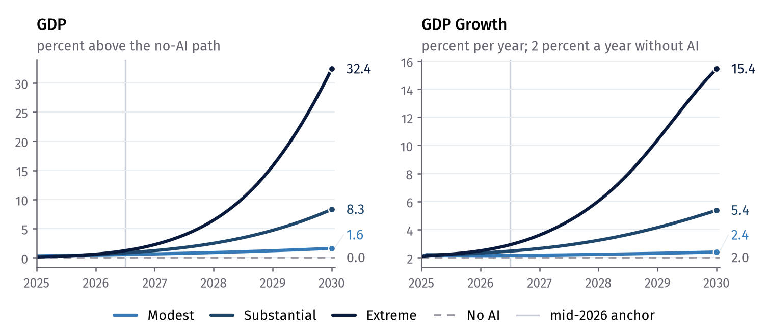
Figure S1:GDP above the path without AI, and GDP growth, in the three scenarios (the paper’s Figure 2).
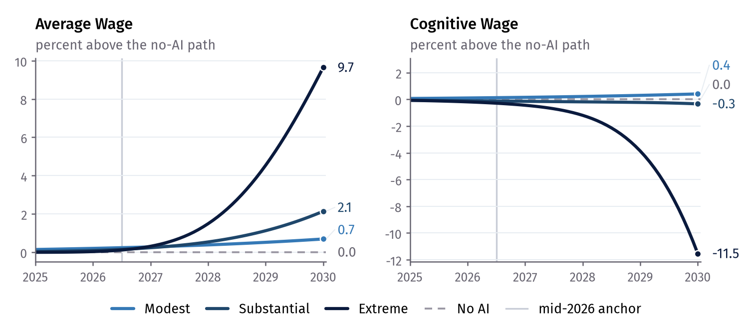
Figure S2:The average wage and the wage in cognitive occupations (the first two panels of the paper’s Figure 3).
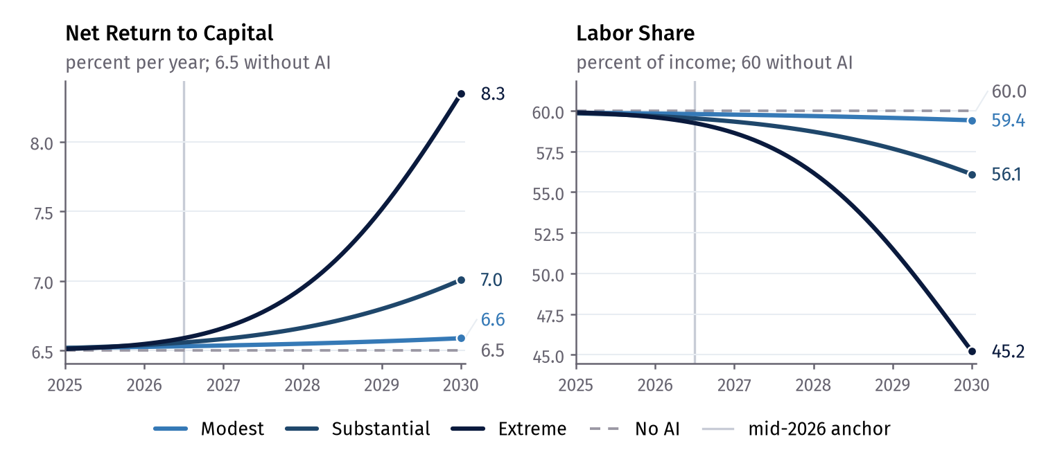
Figure S3:The net return to capital and the labor share (the last two panels of the paper’s Figure 3).
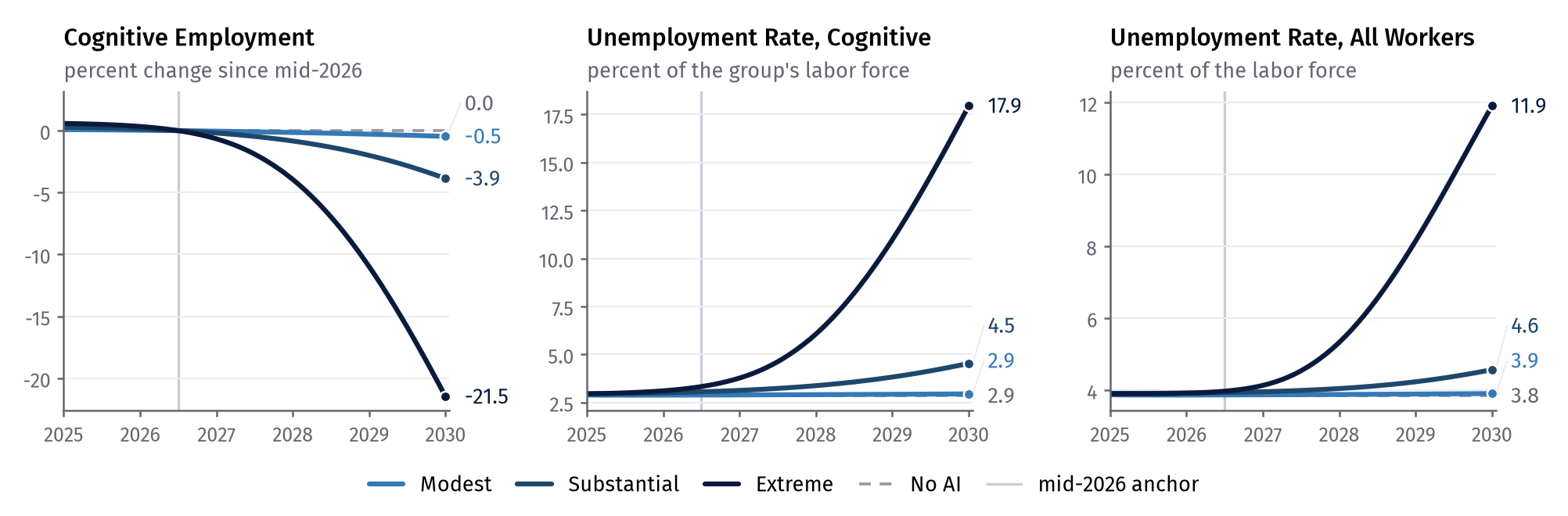
Figure S4:Cognitive employment since mid-2026, the unemployment rate of cognitive workers, and the unemployment rate of all workers (the paper’s Figure 4).
With the same drawing code, the cell below recomputes the three scenarios and redraws Figure S4:
from econ_scenarios import EXTREME, MODEST, SUBSTANTIAL, simulate
from explore import png
from figures import build, figure_panels

runs = {s.name: simulate(s) for s in (MODEST, SUBSTANTIAL, EXTREME)}
png(build(figure_panels(runs["modest"])["figure-4"], runs))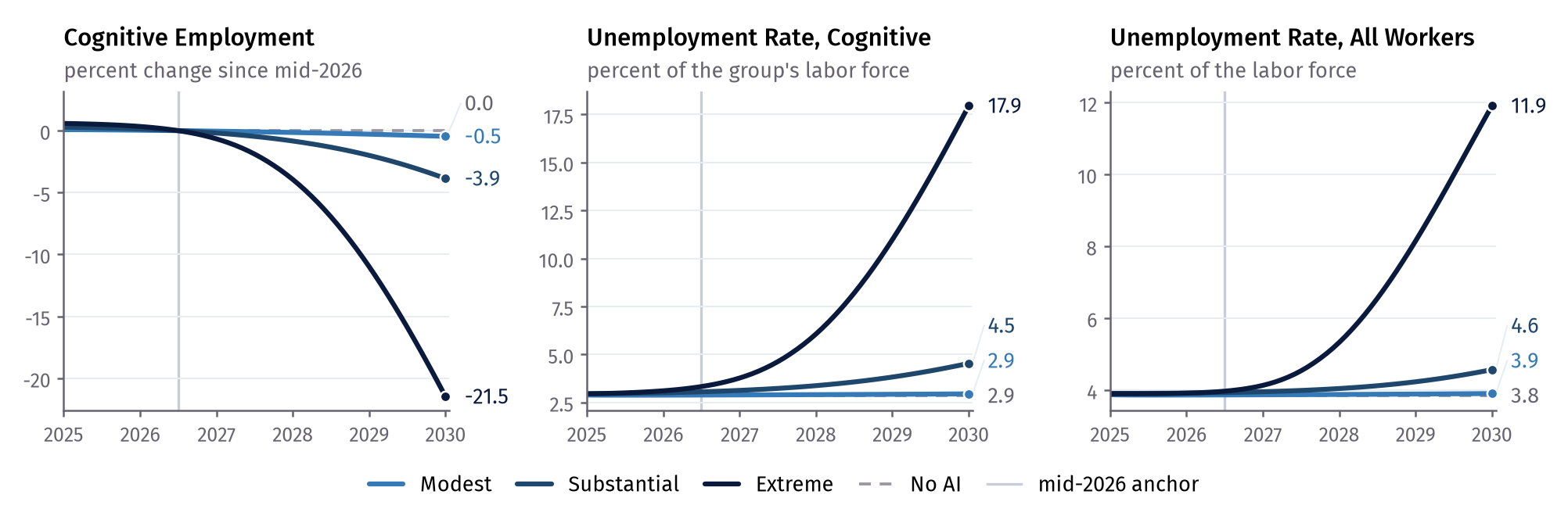
A Cognitive Worker’s View
Because the model tracks each group’s monthly flows between employment and unemployment, the same paths also give one worker’s odds. In Figure S5 we read four of them off the monthly transition matrices: the chance of quitting, the chance of being laid off, the expected length of a spell of unemployment for a worker from cognitive work who is unemployed that month, and the chance that a worker employed in cognitive work is unemployed a year later. Neither the paper nor the explorer displays these odds. Yet they are inputs to any model of household saving, because a worker choosing how much to save must know the chance of losing the job and how long a spell of unemployment would last.
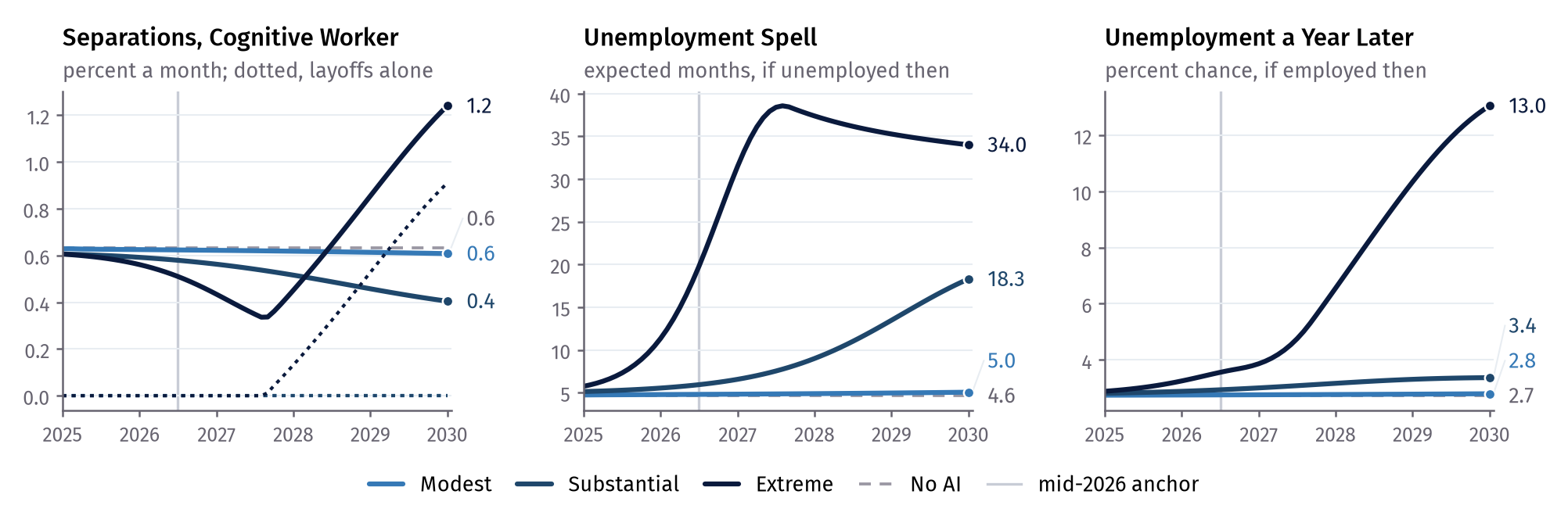
Figure S5:A cognitive worker’s odds, read off the transition matrices. Left: the monthly chance of separating by quit or layoff. Middle: the expected unemployment spell. Right: the chance of being unemployed twelve months later.
To give the two forward-looking measures their full window, I run the simulations behind Figure S5 to 2040, past the figure’s last date; the script code/exhibits.py draws the figure. The table below gives two of these measures for a cognitive worker in January 2029, without AI and in each scenario.
import pages

long_runs = {s.name: simulate(s, horizon=2040.0) for s in (MODEST, SUBSTANTIAL, EXTREME)}
pages.worker_table(long_runs, year=2029.0)A cognitive worker’s odds barely move from those without AI in the modest scenario, while in the extreme scenario an unemployed cognitive worker can expect a spell several times as long and an employed one faces several times the chance of being unemployed a year later.
The Two Checks in Detail
The report’s The Checks states the two checks, their setup, and their results, with the explorer comparison in Figure 1. In the three sections below we recompute every published number at its rounding, run the planted mistakes at full strength, and show which published numbers limit what the second check can detect. The script code/validation/oracle.py downloads and checks the explorer’s JavaScript code and records its outputs, indexed by case, in code/validation/explorer_record.json.gz.
At this point a skeptical reader might object that the first check is circular, since the reimplementation took its calibration record and several definitions from the explorer, so it could have copied the explorer’s mistakes along with its arithmetic. Written from the paper’s text alone, with the explorer’s code withheld, the second implementation of the report’s third comparison suggests that the equations at least were not copied, since it differs from the reimplementation only in the order of the quit conversion once both run on the same data inputs. The inputs themselves are shared, however, and two other checks carry them: the calibration’s public inputs recomputed from their sources in the report’s Table 2, and the fitted numbers the reimplementation reproduces.
The Published Numbers at Their Rounding
The code below recomputes all 226 published numbers and checks each at its printed rounding:
from collections import Counter

from validation.published import cached_runner, checks

results = checks(cached_runner())
for key in ("basis", "role"):
    for value, n in Counter(getattr(c, key) for c in results).items():
        missed = sum(not c.ok for c in results if getattr(c, key) == value)
        print(f"{value:10s} {n:4d} numbers, {missed} outside their rounding")
predicted 211 numbers, 0 outside their rounding
fitted 15 numbers, 0 outside their rounding
output 183 numbers, 0 outside their rounding
input 43 numbers, 0 outside their rounding
The 211 predicted and 15 fitted numbers are those of the summary table above, the 43 inputs those of the inputs subsection, and the 183 outputs what the simulation produces. The six outputs below lie closest to their rounding boundaries, measured as a share of the half-unit their printed rounding allows (0.05 for a number printed to one decimal). Since a planted mistake needs to push these six least before the second check fails, each is likely to be among the first to fail as the mistake grows, although the order also depends on how strongly the mistake moves each published output (Detection Thresholds). Several inputs lie closer still. However, no planted mistake moves an input, so the list leaves the inputs out.
def margin(c):
    """The gap to the rounding boundary, as a share of the half-unit the printed rounding allows."""
    return c.slack / (0.5 * 10.0 ** -c.decimals)


outputs = [c for c in results if c.role == "output"]
for c in sorted(outputs, key=margin)[:6]:
    print(f"{margin(c):.4f}  {c.source}: {c.label}: paper {c.published}, here {c.model:.5f}")
0.0119 Section 2.3.2: unemployment rate of the cognitive group, pct.: paper 2.9, here 2.85060
0.0180 Table 3: Average wage, pct. above the no-AI path [extreme]: paper 9.7, here 9.65090
0.0180 Table 5: wage_avg [extreme, eps=3.0]: paper 9.7, here 9.65090
0.0180 Table 6: wage_avg [extreme, xi=0.5]: paper 9.7, here 9.65090
0.0191 Table 3: Unemployment rate, cognitive workers, pct. [extreme]: paper 17.9, here 17.94905
0.0191 Table 6: unemployment_C [extreme, xi=0.5]: paper 17.9, here 17.94905
Planted Mistakes at Full Strength
At full strength, each of the four planted mistakes of Detection Thresholds makes both checks fail, with the gaps to the explorer that the report gives. The code below runs the published-number check on each planted mistake at full strength and counts the numbers each mistake moves outside their rounding.
from validation.plants import DESCRIPTIONS, PLANTS, planted
from validation.published import failures

for plant in PLANTS:
    with planted(plant) as run:
        missed = failures(cached_runner(run))
    print(f"{DESCRIPTIONS[plant]:36s} {len(missed):3d} published numbers outside their rounding")
quits as the fraction q-hat 8 published numbers outside their rounding
gaps against this month's targets 72 published numbers outside their rounding
first-order rows 65 published numbers outside their rounding
scenario mu in the steady state 65 published numbers outside their rounding
The Binding Published Numbers
Recall that the second check detects a planted mistake only once the mistake pushes some published number past its rounding boundary, so what that check can detect depends on the published numbers closest to their boundaries. Figure S6 shows every output’s margin. For each table the report’s Detection Thresholds names the published numbers that set the smallest mistake the second check can detect there; the figure’s left panel marks those numbers, along with the numbers that fail first as each planted mistake is strengthened.
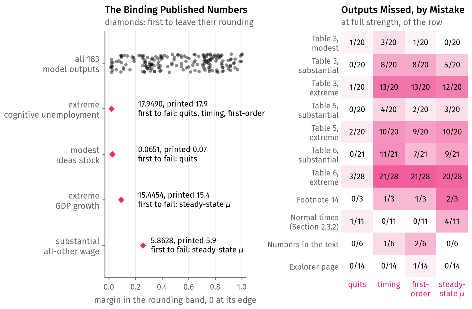
Figure S6:Left: every model output’s margin inside its printed rounding, and the numbers that fail first as each planted mistake is strengthened. Right: the share of each group of outputs that each planted mistake, at full strength, moves outside its rounding.
Further Notes on the Paper and Its Data
The report’s inventory lists the twelve inputs, definitions, and orderings a reimplementation needs beyond the paper’s text. Figure S7 draws the two that move published numbers, the rounded inputs of the paper’s Table 1 and the order in which quit fractions are split and converted to rates, which matching the tables cannot separate from the responsive quit share (the part of normal quitting that rises and falls with job prospects). The four further choices below are parameters and definitions that only matching the published numbers or reading the explorer’s code identifies. Code cells then compute the small differences between the text and the tables that the report describes. The last subsection lists the code behind the report’s recheck of the calibration’s public data.
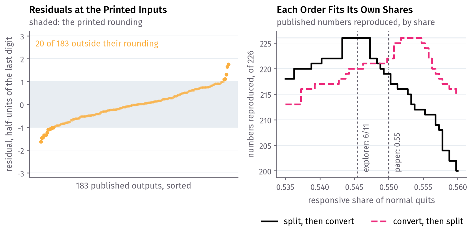
Figure S7:Left: residuals of the 183 published outputs when the model runs on Table 1’s rounded inputs instead of the unrounded record, scaled so that 1 marks the edge of the printed rounding, which is shaded. Right: the number of the 226 published numbers reproduced at each responsive share of normal quits, from 0.535 to 0.560, with quit fractions split before or after Appendix A’s conversion.
In the right panel, under either order the reimplementation reproduces all 226 published numbers on a window of shares that includes values the paper’s Table 1 would print as 0.55. Remarkably, neither window contains 0.55 itself. Matching the tables alone therefore cannot settle the order. However, only the window for the split-first order contains 6/11, the explorer’s value.
Further Choices Taken from the Explorer
System (39) values cognitive labor at its marginal product at realized employment, while the reimplementation records the sticky wage actually paid separately. The gap between that marginal product and the wage paid leaves cognitive employers a profit that reaches, at its largest on any path, 0.3 percent of GDP.
The alternative scenario of Footnote 14 depends on two parameters the footnote does not state. A posting speed of 0.25 and a wage rigidity of 0.5 reproduce its numbers, while a posting speed of 0.5 does not, so these are presumably the values the authors used. Footnote 14’s transfer, the share of the GDP gain that would hold cognitive workers’ income at its level without AI, also depends on the base from which cognitive employment is counted, discussed below.
On its page, the explorer scales the substantial path’s 2025 average GDP to $30.76 trillion and grows it at 2 percent a year, measures the worker split from January 2026 to January 2030, and defines the typical respondent by running Table 2’s median answers through its quiz. These definitions exist only in the explorer’s code.
Like the explorer, the reimplementation bisects the rental-rate gap 100 times and the normal-times steady state 200 times. In its quiz, the explorer also bounds the log gain at (a thirtyfold gain on each AI-performed instance) and the logistic slopes at 3, bounds that
econ_scenariosoffers but does not apply to the paper’s scenarios.
Small Differences between the Text and the Tables
In three places the text and the tables disagree. The report gives the likely reading of each. The cells below compute the numbers behind the three disagreements.
Cognitive Unemployment in Mid-2026
The cell below prints the substantial scenario’s cognitive unemployment rate in 2024, mid-2026, and 2030 beside Section 4.2’s “from 2.9 percent in mid-2026 to 4.5 percent in 2030”, and the rise in the rate measured from each base.
from validation.published import cached_runner, text_table_differences

run = cached_runner()
for c in text_table_differences(run):
    print(f"{c.source}: {c.label}: paper {c.published}, model {c.model:.3f}\n  {c.note}")
Section 4.2: substantial cognitive unemployment in mid-2026, pct.: paper 2.9, model 3.055
the scenario mu applies from 2024, raising the rate before mid-2026; 2.9 is the 2024 steady state, the base the sentence most likely means
Section 4.2: rise in substantial cognitive unemployment from mid-2026 to 2030, pct.: paper 50.0, model 48.422
the sentence says more than 50; from the mid-2026 rate it is 48, from the 2024 rate 59, on which the claim holds
Two Channels in Section 2.1.3
The cell below evaluates Section 2.1.3’s three potential-economy numbers with and without the ideas gain : the wage includes it, the TFP gain leaves it out, and the rental rate rounds to 4.6 either way.
import math

from econ_scenarios import SUBSTANTIAL, Calibration
from econ_scenarios.paths import ScenarioPaths
from econ_scenarios.production import potential, tfp_base_weight

cal = Calibration()
sim = run(SUBSTANTIAL)
k = sim.index(cal.t_read)
x = ScenarioPaths(SUBSTANTIAL, cal).at(cal.t_read)
for label, dlnA in (("with the ideas gain", sim["dlnA"][k]), ("without it", 0.0)):
    p = potential(x, dlnA, cal)
    print(
        f"{label:20s} wage {100 * math.expm1(p.lnW):.2f}, rental rate {100 * math.expm1(p.dlnr):.2f},"
        f" TFP gain {tfp_base_weight(x, dlnA, cal):.3f}"
    )
print(f"{'paper':20s} wage 1.9, rental rate 4.6, TFP gain 0.029")
with the ideas gain wage 1.87, rental rate 4.62, TFP gain 0.030
without it wage 1.71, rental rate 4.57, TFP gain 0.029
paper wage 1.9, rental rate 4.6, TFP gain 0.029
The Base of Footnote 14’s Transfer
The reimplementation reproduces Footnote 14’s transfer of 84 percent of the GDP gain when it counts cognitive employment from mid-2026, and gives 87 percent from the 2024 base of Table 3’s labor-income rows. Since only the mid-2026 base gives 84, that is presumably the base the footnote uses, although its wording, which compares income with its level without AI, reads more naturally on the 2024 base.
Two Points of Notation
The reimplementation and the explorer start the log gain’s line at the mid-2026 anchor at which Table 1 reports , though Equation (8) writes it from the base year of Table A.2. I follow Table A.1’s wage row, which includes the ideas term that Proposition 1’s Equation (16) omits. The report discusses both.
The Public Data behind the Calibration
For each calibration input taken from public data, the reimplementation recomputes the value from its original source, as the report’s Table 2 lists. The code for every row is in code/validation/upstream_*.py. When a source file is missing, its tests fail rather than skip.
Interactive Scenarios
A small version of the authors’ scenario explorer is built below on the reimplementation. Its sliders run in a Python kernel (the process that executes the page’s code cells) that this website cannot yet start in the reader’s browser. The sliders set a scenario’s assumptions from Table 1 of Korinek et al. (2026), plus two calibration numbers (the rigidity of the cognitive wage and the elasticity of capital supply). After each change the cell reruns the model month by month from 2024 and redraws three of the paper’s panels, in which the three published scenarios stay in the background at the paper’s calibration. Until the website can start that kernel, the cell shows a still of the explorer’s first view, the substantial scenario.
import explore

if sys.platform == "emscripten":
    display(explore.Explorer().widget)
else:  # a page built without a browser shows the explorer's first view as a still
    explore.still()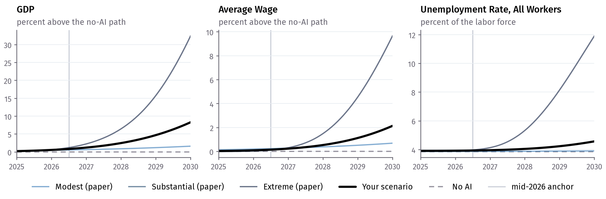
Each slider keeps its assumption inside the range in which the model’s paths are defined, which for the 2030 affected mass lies between its mid-2026 anchor (0.14) and its ceiling (0.624), and for the 2030 diffusion share between 0.10 and 1.
Every number in this section comes from econ_scenarios.simulate, the same function checked against the explorer in the report’s The Checks. Behind the sliders, code/explore.py maps them to a scenario and draws the result.
- Korinek, A., Jones, C. I., Sacher, S., Cotter, T., & McCrory, P. (2026). Economic Scenarios for Transformative AI [Working Paper 2026-02]. The Anthropic Institute. https://www.anthropic.com/institute/econ-scenarios
- Blanchard, O. J., & Galí, J. (2007). Real Wage Rigidities and the New Keynesian Model. Journal of Money, Credit and Banking, 39(s1), 35–65. 10.1111/j.1538-4616.2007.00015.x
- den Haan, W. J., Ramey, G., & Watson, J. (2000). Job Destruction and Propagation of Shocks. American Economic Review, 90(3), 482–498. 10.1257/aer.90.3.482