Abstract
In a risky world, a pessimist assumes the worst; someone who ignores risk is an optimist. Both problems are easy, because pessimist and optimist alike behave as if the world were riskless. A realist, responding optimally to risk, spends between the two. We use that to change what is interpolated: not consumption, but the logit of a moderation ratio recording where between the two rules the realist lies. The result cannot escape the bounds the two rules form, is accurate on five gridpoints, and beyond the last of them is more than an order of magnitude more accurate than the endogenous gridpoints method. It carries over to value and to risky returns, and to the portfolio share with the logarithm in place of the logit.
Key Points
A realist’s consumption lies between a pessimist’s rule and an optimist’s
Interpolating the logit of where it lies keeps the approximation inside both bounds
Five gridpoints suffice, and beyond them the method is ten times as accurate as EGM
The bracket carries over to value, artificial constraints, risky returns, and assets
For the portfolio share the log of the moderation ratio replaces the logit
1Introduction
Solving a consumption, investment, portfolio choice, or similar intertemporal optimization problem using numerical methods generally requires the modeler to choose how to represent a policy or value function. In the stochastic case, where analytical solutions are generally not available, a common approach is to use low-order polynomial splines that exactly match the function (and maybe some derivatives) at a finite set of gridpoints, and then to assume that interpolated or extrapolated versions of that spline represent the function well at the continuous infinity of unmatched points. Outside the range of the gridpoints, however, this trust is often misplaced Ma & Toda, 2022White, 2015, and extending the grid does not restore it, because beyond whatever gridpoint is last a linearly extrapolated consumption rule eventually predicts negative precautionary saving, which theory rules out for any prudent consumer.
This paper argues that a better approach is to rely upon the fact that without uncertainty, the optimal consumption function has a simple analytical solution. The key insight is that, under standard assumptions, the consumer who faces an uninsurable labor income risk will consume less than a consumer with the same path for expected income but who does not perceive any uncertainty. The ‘realist’ consumer, who does perceive the risks, will engage in ‘precautionary saving’ Leland, 1968Sandmo, 1970Kimball, 1990, so the perfect foresight riskless solution provides an upper bound to the solution that will actually be optimal. A lower bound is provided by the behavior of a consumer who has the subjective belief that the future level of income will be the worst that it can possibly be. This consumer, too, behaves according to the convenient analytical perfect foresight solution, but their certainty is that of a pessimist perfectly confident in their pessimism. The realist’s consumption lies strictly between these two immoderate benchmarks. We use this fact to change the object being interpolated, so that rather than consumption itself we interpolate a moderation ratio that measures where the realist falls between the pessimist and the optimist. Because that ratio is bounded and smooth and its logit is asymptotically linear, the logit interpolates and extrapolates far more accurately than when the level of the consumption ratio is approximated, and by construction the result can never violate the bounds.
On a standard calibration the method is more accurate than the benchmark endogenous gridpoints method (EGM) in every interval between gridpoints, and by more than an order of magnitude in all but the first. Beyond the last gridpoint, where EGM’s default linear extrapolation fails outright, it is roughly forty-six times more accurate over the range we evaluate, and even when EGM is lent the same bounds to hold its extrapolation inside them, it remains less accurate there, by a factor of seventeen.
We build on bounds for the consumption function and limiting marginal propensities to consume established in buffer-stock theory Stachurski & Toda, 2019Ma et al., 2020Carroll, 2009Ma & Toda, 2021 for the standard buffer-stock problem Carroll, 1997. Using results from Carroll & Shanker (2026), we show how to use these upper and lower bounds to tightly constrain the shape and characteristics of the solution to the problem of the ‘realist.’ Imposition of these constraints can clarify and speed the solution of the realist’s problem.[1]
After showing how to use the method in the baseline case, we show how to refine it to encompass an even tighter theoretical bound, and how to extend it to solve a problem in which the consumer faces both labor income risk and rate-of-return risk. Section 2 states the realist’s problem and the patience conditions that guarantee a finite solution, and Section 3 sets out the endogenous gridpoints benchmark. Section 4 develops the method of moderation for the consumption function and, in Section 4.3, for the value function; Section 5 quantifies its accuracy against endogenous gridpoints; and Section 6 takes up four extensions: the tighter bound near the borrowing constraint (Section 6.1), Hermite interpolation that matches the Euler equation at each gridpoint (Section 6.2), an artificial borrowing constraint (Section 6.3), and a problem stated in assets rather than market resources (Section 6.4). Section 7 makes the return risky and then makes the risky share a choice, which is where the method first meets a bound that the solution actually reaches at a finite level of wealth instead of merely approaching.
2The Realist’s Problem
The truly optimal behavior in the problem facing the consumer who understands all their risks is captured by
where the utility function is CRRA with risk aversion parameter :
Maximization is subject to the budget constraints
where the variables are defined as
The exogenous variables evolve according to the Friedman-Muth Income Process[2]:
where is the deterministic permanent income growth factor, and the permanent shocks to income are independently and identically distributed with mean and support where .[3] The worst transitory draw arrives with probability . The Friedman-Muth unemployment case sets ; a positive is the same unemployment event paying a benefit, which leaves income at a positive floor rather than at zero. Everything below requires only that is indeed the worst draw, , which holds automatically when . Transitory shocks other than the worst draw, , are independently distributed with mean and bounded support where ; the scaling factor in (5) keeps .
It turns out (see Carroll (2020) for a proof) that this problem can be rewritten in a more convenient form in which choice and state variables are normalized by the level of permanent income, e.g., using nonbold font for normalized variables, . When that is done, the Bellman equation for the transformed version of the consumer’s problem is
and because we have not imposed a liquidity constraint, the solution satisfies the Euler equation
We define the absolute patience factor , the factor by which a perfect foresight consumer’s consumption grows from one period to the next. Whether the problem has a well-behaved solution depends on a set of conditions established and named in Carroll & Shanker (2026), whose names we adopt and whose content we state here, because we appeal to them repeatedly below.
Three conditions govern the solution. The finite value of autarky condition (FVAC), , says that a consumer who simply consumed their income in every period (‘autarky’) would obtain finite lifetime value, so that the objective being maximized is finite to begin with. The absolute impatience condition (AIC), , says that the perfect foresight consumer plans a falling rather than a rising consumption path; it is what makes the consumer want to run a buffer stock down rather than accumulate without limit. The return impatience condition (RIC), , says that planned consumption growth falls short of the rate at which resources accumulate, so the perfect foresight consumer spends a strictly positive fraction of their resources ( in (9) below) instead of deferring spending indefinitely.
Two further conditions relate spending to the growth of income. The growth impatience condition (GIC), , says that consumption grows more slowly than permanent income, which is what makes the ratio of wealth to permanent income revert to a target instead of drifting away. The finite human wealth condition (FHWC), , says that the present discounted value of future labor income is finite, so that the ‘optimist’ rule we construct below exists at all.
Together these conditions ensure existence of the upper and lower bounds on consumption that the method of moderation is built from Carroll, 2009Stachurski & Toda, 2019 and pin down the limiting MPCs Ma & Toda, 2021.
We simplify the exposition by setting and assuming with probability 1 for all (no permanent income growth or shocks), and drop time subscripts except where context requires, working with the infinite-horizon formulation.[4] Under these simplifications, FVAC becomes , the GIC coincides with the AIC, and the FHWC reduces to . All results apply equally to finite-horizon models via backward recursion from terminal period , and to models with permanent income growth by appropriately adjusting the patience conditions above. The generalization to the case with permanent shocks is straightforward.[5]
3Benchmark: The Method of Endogenous Gridpoints
For comparison to our new solution method, we use the endogenous gridpoints solution to the microeconomic problem presented in Carroll (2006). That method computes the level of consumption at a set of gridpoints for market resources that are determined endogenously using the Euler equation. The consumption function is then constructed by linear interpolation among the gridpoints thus found. Extensions of this method handle multi-dimensional problems Barillas & Fernández-Villaverde, 2007, occasionally binding constraints Hintermaier & Koeniger, 2010, non-smooth and non-concave problems Fella, 2014, and discrete-continuous choice models Iskhakov et al., 2017, while White (2015) treats the method’s theory and practice. None of them repairs behavior outside the solved grid, which is the problem we take up here. The closest work on that problem takes a different route, since Ma & Toda (2022) justify linearly extrapolating consumption itself at its asymptotic MPC, and Gouin-Bonenfant & Toda (2023) build wealth-tail analysis on the same asymptotics. Extrapolating the level enforces the correct slope only in the limit, whereas the method below extrapolates a bounded transform, which keeps the approximation between both theoretical bounds at every finite wealth level whatever slope the boundary supplies.
Carroll (2020) describes a specific calibration of the model and constructs a solution using five gridpoints chosen to capture the structure of the consumption function reasonably well at values of near the infinite-horizon target value (See those notes for details). The five gridpoints are for illustration (applied work typically uses 30-80 gridpoints for accurate solutions), and the comparisons below show what happens to each method when the grid is this sparse.
Throughout the numerical illustrations we adopt this calibration: relative risk aversion , discount factor , and gross risk-free return , with no permanent income growth or shocks (, ) and mean-one transitory shocks of log standard deviation 1 discretized on a seven-point equiprobable grid (the quadrature schemes of Tauchen (1986) and Tauchen & Hussey (1991) are the standard alternatives). The calibration has no zero-income atom, since the worst draw is the smallest point of the (strictly positive) discretized grid, so the general worst-shock case of (5) applies with equal to that point’s probability, and the natural borrowing constraint is negative. Unless otherwise noted, the figures and the accuracy comparison below display the next-to-last period of the finite-horizon problem, for which the analytical last-period rule furnishes exact boundary conditions (human wealth one period before the end is , in contrast to the infinite-horizon value of 50), and both methods use linear interpolation, of consumption for endogenous gridpoints and of the logit for moderation. The Hermite refinement is treated separately in Section 6.2.
The endogenous gridpoints solution method says nothing about how the policy function should be extrapolated beyond the grid at which the problem has been solved, and that silence allows many interpretations. Here we assume the natural choice of linear extension, which leads to badly wrong outcomes. (Other common solution methods are no better outside their own predefined ranges.) Figure 1 demonstrates the point by plotting the amount of precautionary saving implied by a linear extrapolation of our approximated consumption rule (the consumption of the perfect foresight consumer minus our approximation to optimal consumption under uncertainty, ). Although theory proves that precautionary saving is always positive, the linearly extrapolated numerical approximation eventually predicts negative precautionary saving (at the point in the figure where the extrapolated locus crosses the horizontal axis).
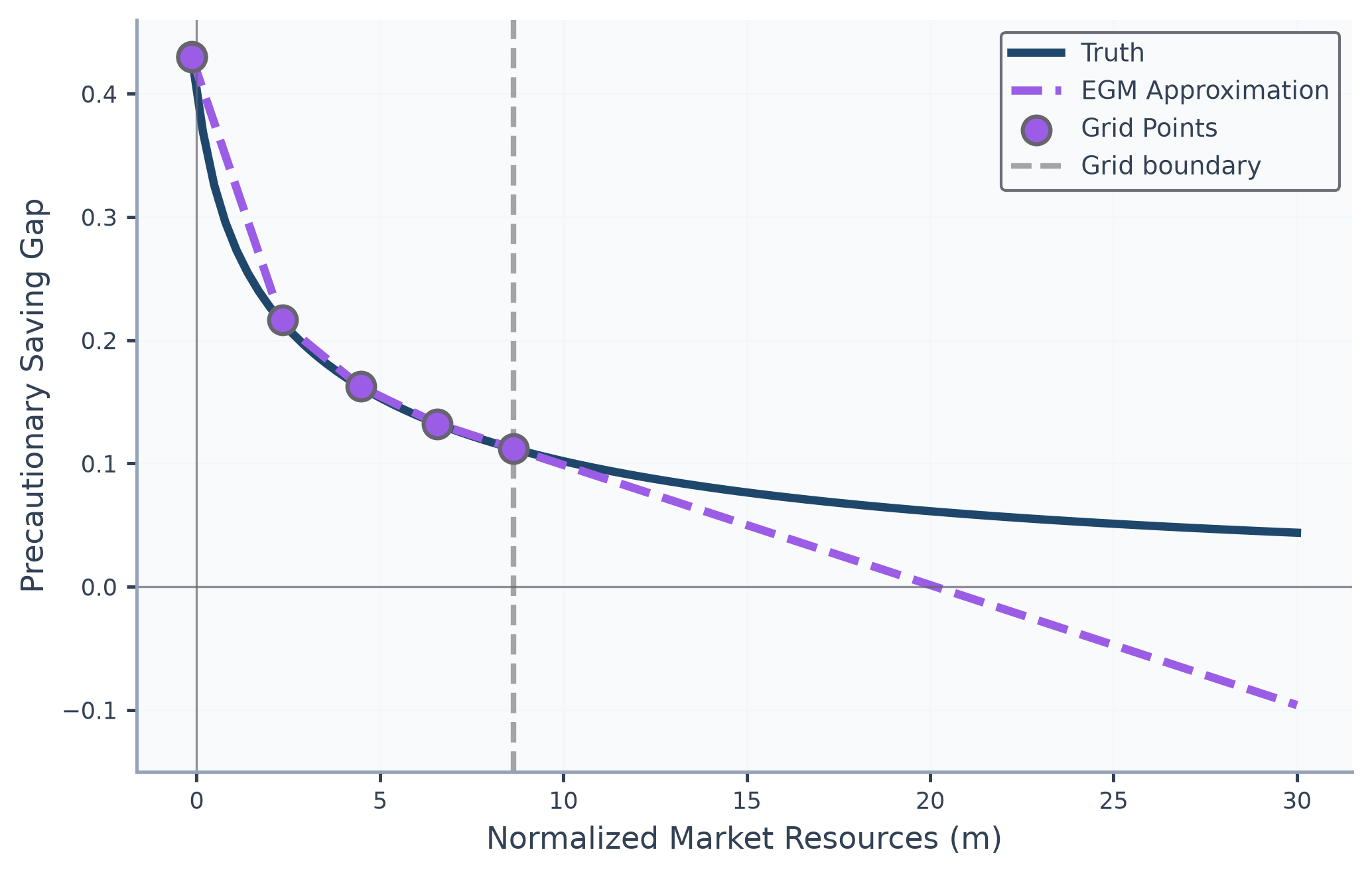
Figure 1:For Large Enough , Predicted Precautionary Saving is Negative (Oops!)
This error cannot be fixed by extending the upper gridpoint; in the presence of serious uncertainty, the consumption rule will need to be evaluated outside of any prespecified grid (because starting from the top gridpoint, a large enough realization of the uncertain variable will push next period’s realization of assets above that top; a similar argument applies below the bottom gridpoint). While a judicious extrapolation technique can prevent this problem from being fatal (for example by carefully excluding negative precautionary saving), the problem is often dealt with using inelegant methods whose implications for the accuracy of the solution are difficult to gauge. A fix chosen because it is convenient can restore the sign of precautionary saving while leaving its magnitude ungrounded in the theory, which matters because the convenient fixes are the ones a modeler tries first.[6]
4The Method of Moderation
4.1The Optimist, the Pessimist, and the Realist
As a preliminary to our solution, define as end-of-period human wealth (the present discounted value of future labor income) for a perfect foresight version of the problem of a ‘risk optimist:’ a consumer who believes with perfect confidence that the shocks will always take their expected value of 1, for all . Under the FHWC this present value converges to , which is in our calibration with . The solution to a perfect foresight problem of this kind takes the form[7]
for a constant minimal marginal propensity to consume, which in the infinite-horizon case is
strictly positive under the RIC.[8] We similarly define as ‘minimal human wealth,’ the present discounted value of labor income if the shocks were to take on their worst value (zero for uninsured unemployment, positive when unemployment pays a benefit) in every future period, for all (which we define as corresponding to the beliefs of a ‘pessimist’). The same limit gives , which is zero when the worst shock is unemployment.
We will call a ‘realist’ the consumer who correctly perceives the true probabilities of the future risks and optimizes accordingly.
For the realist, a lower bound for the level of market resources is , because if equalled this value then there would be a positive finite chance (however small) of receiving in every future period, which would require the consumer to set to zero to guarantee that the intertemporal budget constraint holds. Since consumption of zero yields infinite marginal utility, the solution to the realist consumer’s problem is not well defined for values of Zeldes, 1989Deaton, 1991, and the limiting value of the realist’s is zero as .
Given this result, it will be convenient to define ‘excess’ market resources as the amount by which actual resources exceed the lower bound, and ‘excess’ human wealth as the amount by which mean expected human wealth exceeds guaranteed minimum human wealth:[9]
We can now transparently define the optimal consumption rules for the two perfect foresight problems, those of the ‘optimist’ and the ‘pessimist.’ The ‘pessimist’ perceives human wealth to be equal to its minimum feasible value with certainty, so consumption is given by the perfect foresight solution
The ‘optimist,’ on the other hand, pretends that there is no uncertainty about future income, and therefore consumes
4.2The Consumption Function
It seems obvious that the spending of the realist will be strictly greater than that of the pessimist and strictly less than that of the optimist. The realist reoptimizes as uncertainty resolves, while the pessimist must finance every future period out of saving, and because the adverse outcome remains possible, even a wealthy realist is never completely self-insured. Figure 2 illustrates the proposition for the consumption rule in period .
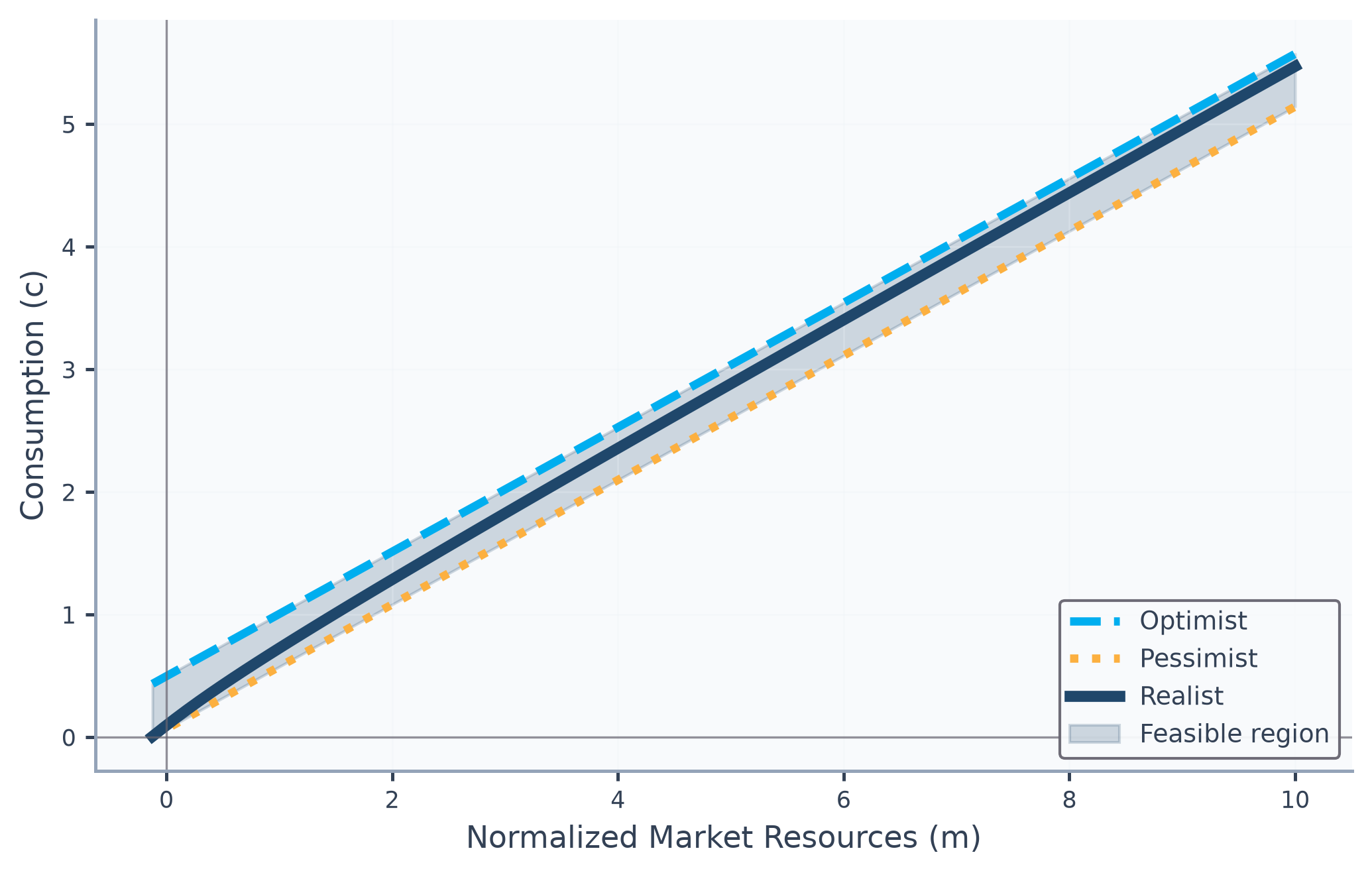
Figure 2:Moderation Illustrated:
The proof is more difficult than might be imagined, but the necessary work is done in Carroll & Shanker (2026): under shocks with nondegenerate bounded support (whose worst realization may be zero), the consumption function is strictly increasing and concave Carroll & Kimball, 1996 and lies strictly between the two perfect foresight rules. We therefore take the proposition as a fact and proceed by manipulating the inequality:
Subtracting in each of these inequalities and using Equations (11) and (12) gives
where the fraction in the middle of the last inequality is the moderation ratio measuring how close the realist’s consumption is to the optimist’s behavior (the numerator is the gap between the realist and pessimist) relative to the maximum possible gap between optimist and pessimist. When , the realist behaves like the pessimist (maximum precautionary saving); when , the realist behaves like the optimist (no precautionary saving). Under bounded shocks neither endpoint is attained, so lies strictly inside for all , and the equivalent form places the realist strictly between the pessimist and the optimist.
Figure 3 shows why we work in this quantity rather than in consumption itself. The bracket has a constant width of , so in levels it shrinks against the rule it brackets, from more than half of the optimist’s consumption near the constraint to under a tenth by , which is why the three agents of Figure 2 crowd onto one line. The same information rescaled by that width fills its range, as climbs from zero at the constraint through 0.5 near and past 0.8 by , with the five gridpoints spread across the climb rather than bunched.
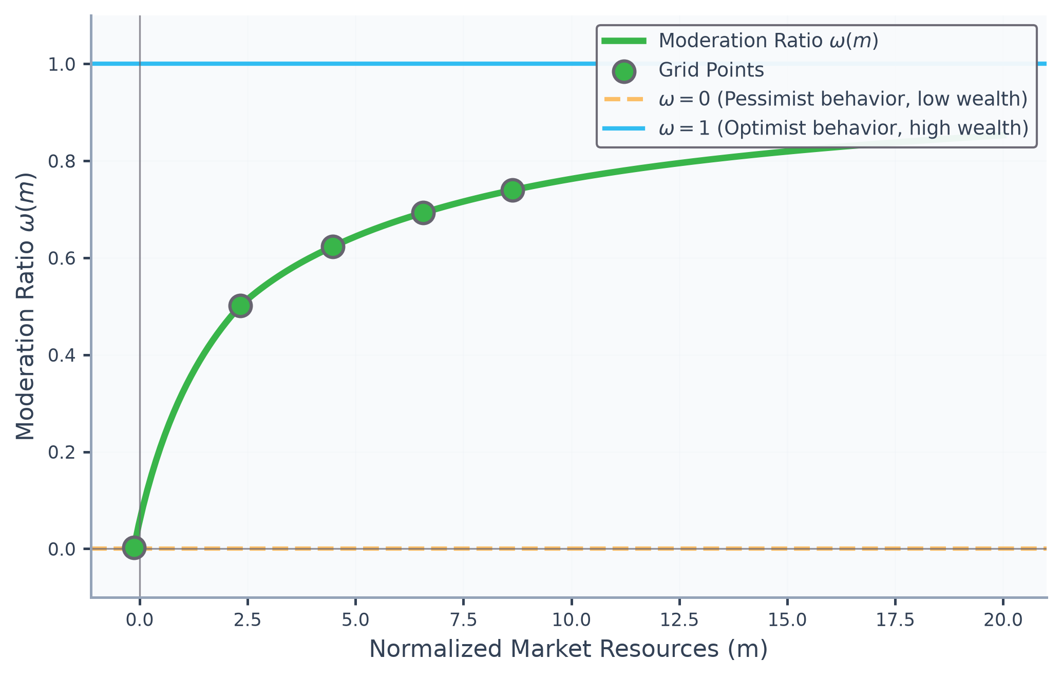
Figure 3:Rescaling by the Bracket Width Turns a Vanishing Gap Into a Full-Range Object
Defining (which can range from to ), the object in the middle of the last inequality is
and we now define
which carries the bounded moderation ratio to the whole real line, just as the log carried to . The inverse is the sigmoid , with as the realist approaches the optimist and as the realist approaches the pessimist.
The transformed function suits linear interpolation because it straightens at both ends of its domain. As the realist’s MPC approaches a finite limit above (the bound of Section 6.1), hence vanishes in proportion to and approaches a line with slope one. As , is asymptotically linear,[10] so we extrapolate it linearly using the slope at the upper boundary gridpoint. Because any linear extrapolation of the logit maps back through the sigmoid into , the approximation satisfies throughout the extrapolation domain. Equation (16) splits the logit into two pieces, and , and either piece alone would enforce only one of the two bounds.
Each piece straightens the tail at which its own bound is approached, where and where . Here both bounds are approached only asymptotically, the pessimist’s as and the optimist’s as , so both singularities of the logit lie at the ends of the domain. The logit needs bounds that are approached and never reached, though it does not care from which side, since reorienting the ratio only changes the sign of the transform, . Where a bound is actually reached at some finite level of wealth, the piece belonging to it diverges at the edge of the working range, and instead of straightening the approach it bends it, so the right transform there is the one-sided piece for the bound that is only approached. The portfolio share below presents exactly that case.
Figure 4 plots the object the method actually interpolates: for the five-gridpoint solution of the calibration above. The function is smooth, gently curved in the middle of the grid, and close to linear at both ends.
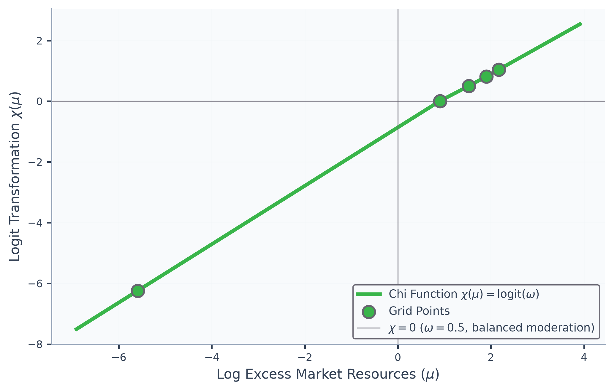
Figure 4:The Interpolated Object Is Smooth and Close to Linear at Both Ends
Given , the consumption function can be recovered from
Thus, the procedure is to calculate at the points corresponding to the log of the points defined above, and then using these to construct an interpolating approximation from which we indirectly obtain our approximated consumption rule (an approximation to the true ) by substituting for in Equation (17).
Because this method relies upon the fact that the problem is easy to solve if the decision maker has unreasonable views (either in the optimistic or the pessimistic direction), and because the correct solution is always between these immoderate extremes, we call our solution procedure the ‘method of moderation.’
Figure 5 is visually indistinguishable from the true rule; a reader with very good eyesight might detect the barest hint of a discrepancy between the Truth and the Approximation at the far right-hand edge of the figure, a stark contrast with the calamitous divergence evident in Figure 1.
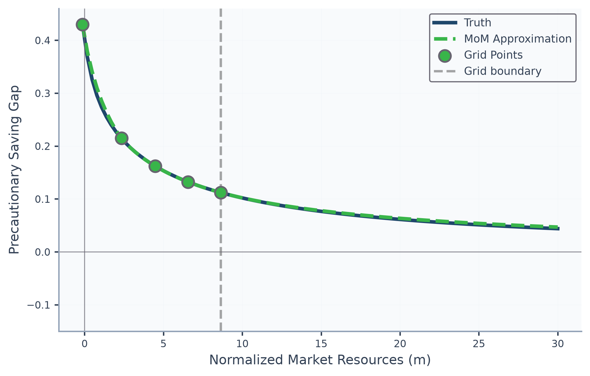
Figure 5:Extrapolated Stays on the True Rule Where Linear EGM Extrapolation Diverged
4.3The Value Function
Often it is useful to know the value function as well as the consumption rule. Fortunately, many of the tricks used when solving for the consumption rule have a direct analogue in approximation of the value function.
Consider the perfect foresight (or “optimist’s”) problem in period . Using the fact that in a perfect foresight model the growth factor for consumption is constant, we can use to calculate the value function in period :
where is the present discounted value of consumption, normalized by current consumption. Using the fact demonstrated in Carroll & Shanker (2026) that [11], a similar function can be constructed recursively for earlier periods, yielding the general expression
This can be transformed as
The transformation applies the inverse utility function to value, , expressing value in consumption units. Despite the customary name ‘inverse value function,’ it is this composition, not the functional inverse of itself. The pessimist’s inverse value follows by the same steps, with :
hence , the denominator that normalizes the value moderation ratio in (23) below.
We apply the same transformation to the value function for the problem with uncertainty (the “realist’s” problem):
and the value function can be approximated by calculating the values of at the same gridpoints used by the consumption function approximation, and interpolating among those points.
However, as with the consumption approximation, we can do even better if we realize that the function for the optimist’s problem is an upper bound for the function in the presence of uncertainty, and the value function for the pessimist is a lower bound. The ordering holds because the realist’s true income process stochastically dominates the pessimist’s worst-case income and is dominated, for a risk-averse agent, by the optimist’s certain expected income. Because the inverse-value transform is monotonic, the same ordering carries over to . Analogously to (15), define an upper-case
and an upper-case version of the equation in (16):
and if we approximate these objects then invert them (as above with the and functions) we obtain an approximation to the inverted value function that respects both bounds by construction, at the same points for which we have our approximated value function:
from which we obtain our approximation to the value function as
5Numerical Accuracy
The figures show the failure and the repair but not the size of the gain, so we compare the method of moderation against the benchmark endogenous gridpoints method on the calibration above, solving both on the same sparse five-point grid. We report in Table 1 the maximum absolute consumption error on a dense subgrid of each interval between adjacent gridpoints , and of the extrapolation region running out to , taking a high-precision endogenous gridpoints solution (500 gridpoints) as the truth. The moderation column applies the near-constraint envelope of Section 6.1, which is slack over the tabulated range under the natural constraint used here. Except in the first interval, where the advantage is about three and a half times, the method of moderation is more than an order of magnitude more accurate than EGM, and we obtain this on a fixed sparse grid without optimizing the grid itself Chipeniuk, 2020. The contrast is starkest in the extrapolation region beyond the top gridpoint, exactly where Figure 1 showed linear EGM extrapolation failing, and there the method of moderation is roughly forty-six times more accurate. That ratio is a property of the horizon as much as of the two methods, since EGM’s linear extrapolation diverges and any ratio one likes can be had by evaluating far enough out. The fairer comparison, against an EGM rule handed the same bounds, is seventeen, and we come to it below.[12]
Table 1:Maximum approximation errors by interval for endogenous gridpoints (EGM) and the method of moderation (MoM) on the same five-point grid with linear interpolation: absolute consumption errors against the reference solution (upper panel) and the largest Euler-equation residual in consumption-equivalent units, which needs no reference solution (lower panel). Gridpoints , , , , ; evaluation horizon . Orders of magnitude in parentheses.
| Method | |||||
| Absolute error | |||||
| EGM | 5.4(-2) | 4.2(-3) | 1.6(-3) | 8.6(-4) | 1.4(-1) |
| MoM | 1.5(-2) | 2.5(-4) | 1.4(-4) | 7.4(-5) | 3.0(-3) |
| Euler residual | |||||
| EGM | 7.7(-1) | 4.6(-3) | 1.1(-3) | 4.2(-4) | 1.8(-2) |
| MoM | 1.7(-1) | 2.7(-4) | 9.8(-5) | 3.6(-5) | 4.1(-4) |
Figure 6 shows that the table’s intervals are error humps, with both approximations nearly exact at the sparse gridpoints and less accurate between them, and the method of moderation’s humps sit below EGM’s throughout. The two methods part company beyond the top gridpoint (marked), where the EGM error rises steeply as its linear extrapolation drifts away from the truth, whereas moderation stays flat.
An absolute error is hard to interpret near the borrowing constraint, where consumption itself is close to zero, so in the lower panel of the table we score the same two rules by a yardstick that depends neither on the scale of consumption nor on our reference solution: the Euler-equation residual, the proportion by which consumption would have to change for the Euler equation to hold exactly Santos, 2000. By the residual, as by the absolute errors, the method of moderation is more accurate in every interval, by a factor of four and a half in the first, eleven to seventeen in the interior, and forty-four beyond the top gridpoint. Both methods do poorly in the first interval by this yardstick, since near the constraint even a small absolute error is a large proportion of consumption.
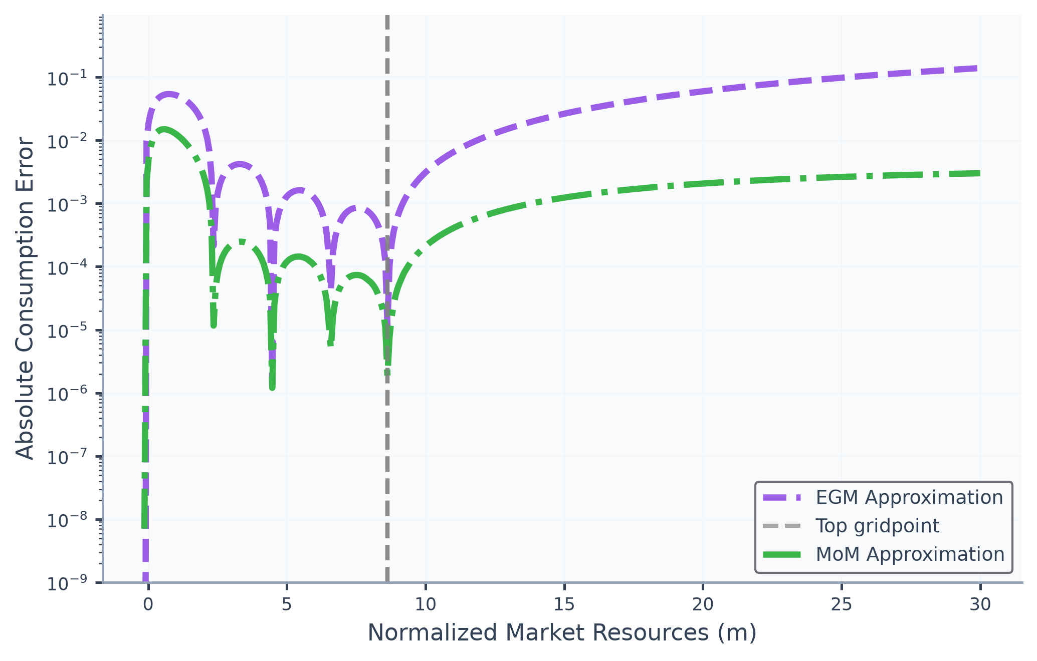
Figure 6:Moderation’s Error Humps Sit Below EGM’s Between Gridpoints and Stay Flat Beyond the Top Gridpoint
The two halves of the figure have different causes. Inside the grid we gain because is the smoother object, and beyond it because linear extrapolation of cannot leave the bracket, while linear EGM extrapolation eventually does.
Grid design governs beyond-grid accuracy but never the bounds, and what matters is how far the grid reaches rather than how many points it holds (Figure 7). Raising the count from five to thirty without moving the top gridpoint does not improve the beyond-grid error at all, while moving the top out to twice human wealth improves it by roughly an order of magnitude, and to four times human wealth by a further factor of two; the two spacings the figure plots differ little by comparison. In practice we would therefore pair the 30-80 gridpoints noted earlier with a top gridpoint at a small multiple of human wealth, which the exhibits above already satisfy, human wealth one period before the end being close to one.
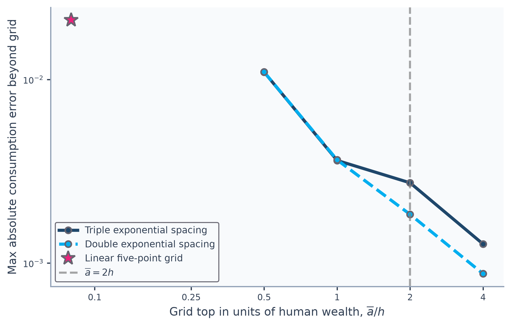
Figure 7:Extending the Grid Top Improves Beyond-Grid Accuracy, While the Bounds Hold Everywhere
A skeptical reader will want to know how much of the comparison of Table 1 is the design rather than the method, so we ran two further comparisons. First, on a grid of the size used in practice (twenty points, triple-exponential spacing, same top gridpoint) both methods gain roughly two orders of magnitude of interior accuracy, compressing moderation’s worst-case interior advantage to about four times (the median interval ratio is eleven), while beyond the grid the ratio is untouched by refinement, forty-six at five points and at twenty. Second, the extrapolation advantage does not come from denying EGM the bounds, for when we impose the same optimist and pessimist bounds on EGM’s rule every interior interval is unchanged (neither bound binds inside the grid) and its beyond-grid error falls only from 1.4(-1) to 6.1(-2), against 3.0(-3) for moderation. Nor does that comparison depend on the evaluation horizon . The error of EGM without the bounds grows without limit as the horizon extends, but the errors of the bounded EGM rule and of moderation both level off, at 6.1(-2) and 3.6(-3), so their ratio converges to seventeen however far the comparison runs. Imposing the bounds also concedes the premise, since the bounds EGM borrows are exactly what the method of moderation is built on, and the bounded rule is kinked wherever a bound binds, whereas moderation approaches its bounds smoothly by construction.
6Extensions
6.1A Tighter Upper Bound
Carroll & Shanker (2026) derives an upper limit for the MPC as approaches its lower bound. Recalling that is the probability of the worst income draw, (one seventh in the calibration above, where the worst draw is one point of a seven-point equiprobable grid), the infinite-horizon limit is
which nests the Friedman-Muth unemployment case of Carroll & Toche (2009).[13] Using this fact plus the strict concavity of the consumption function yields the proposition that
Near the constraint the optimist’s bound is loose, because it is calibrated to the low MPC that prevails at high wealth. Moderating between the two perfect-foresight rules alone therefore does not guarantee that approximated consumption will respect this tighter constraint between gridpoints, and a failure to respect it can occasionally cause computational problems in solving or simulating the model. Here, we describe a method for constructing an approximation that always satisfies the constraint. It is applied throughout, so every consumption number reported in this paper respects the tighter bound, except where we drop the envelope on purpose to show what it does.
Defining as the cusp point where the two upper bounds intersect (where ):
this intersection occurs in the feasible region (), because under the stated conditions and so .
The two bounds therefore change places at , the tighter bound binding below it and the optimist’s above it. Since the realist’s rule respects both everywhere, it respects whichever is smaller,
and we build the approximation to respect it too, by taking the same lower envelope of the moderated rule and the tighter bound. This just says that at each level of wealth we use whichever of the two is the more appropriate, without needing to know in advance which that will be.
Doing so cannot make the approximation worse, because where the moderated rule already lies below the tighter bound, the envelope leaves it alone. If instead the rule lies above the bound, the truth lies below it, so the bound is closer than the moderated value was. At wealth levels where the constraint actually binds, the envelope is not an approximation at all, because there the realist consumes exactly.[14]
This is the lower-envelope construction Carroll & Shanker (2026) use for a liquidity constraint, with the constrained branch in closed form joined to the unconstrained branch. The bound imposed here is , which for lies strictly inside the budget line .
We now construct an upper-bound value function, denoted to distinguish it from the optimist’s own value , implied for a consumer whose spending behavior is consistent with the refined upper-bound consumption rule.
For , the refined consumption rule coincides with the optimist’s, so there we set . However, for values , matters are slightly more complicated.
Start with the fact that at the cusp point,
For every , value equals current utility plus a continuation term,
where is the end-of-period value as a function of the assets retained at the end of the period. Below the cusp point the refined rule spends , which leaves assets of , so for
which can be computed directly because , where is the growth-normalized gross return and is as defined above, because a consumer who ends the current period with assets exceeding the lower bound will not expect to be constrained next period. (Recall again that we are merely constructing an object that is guaranteed to be an upper bound for the value that the ‘realist’ consumer will experience. When the worst draw is unemployment, and the retained-asset expression reduces to .) At the gridpoints defined by the solution of the consumption problem we can then construct
which yields the appropriate vector for constructing and . The rest of the procedure mirrors the one performed for the consumption rule, and delivers a value-function approximation that respects the tighter bound below the cusp and the optimist’s bound above it.
Figure 8 shows why the refinement is worth the trouble. To the left of the cusp the optimist’s rule permits spending the realist would never choose, and only the tighter bound keeps the approximation out of that region.
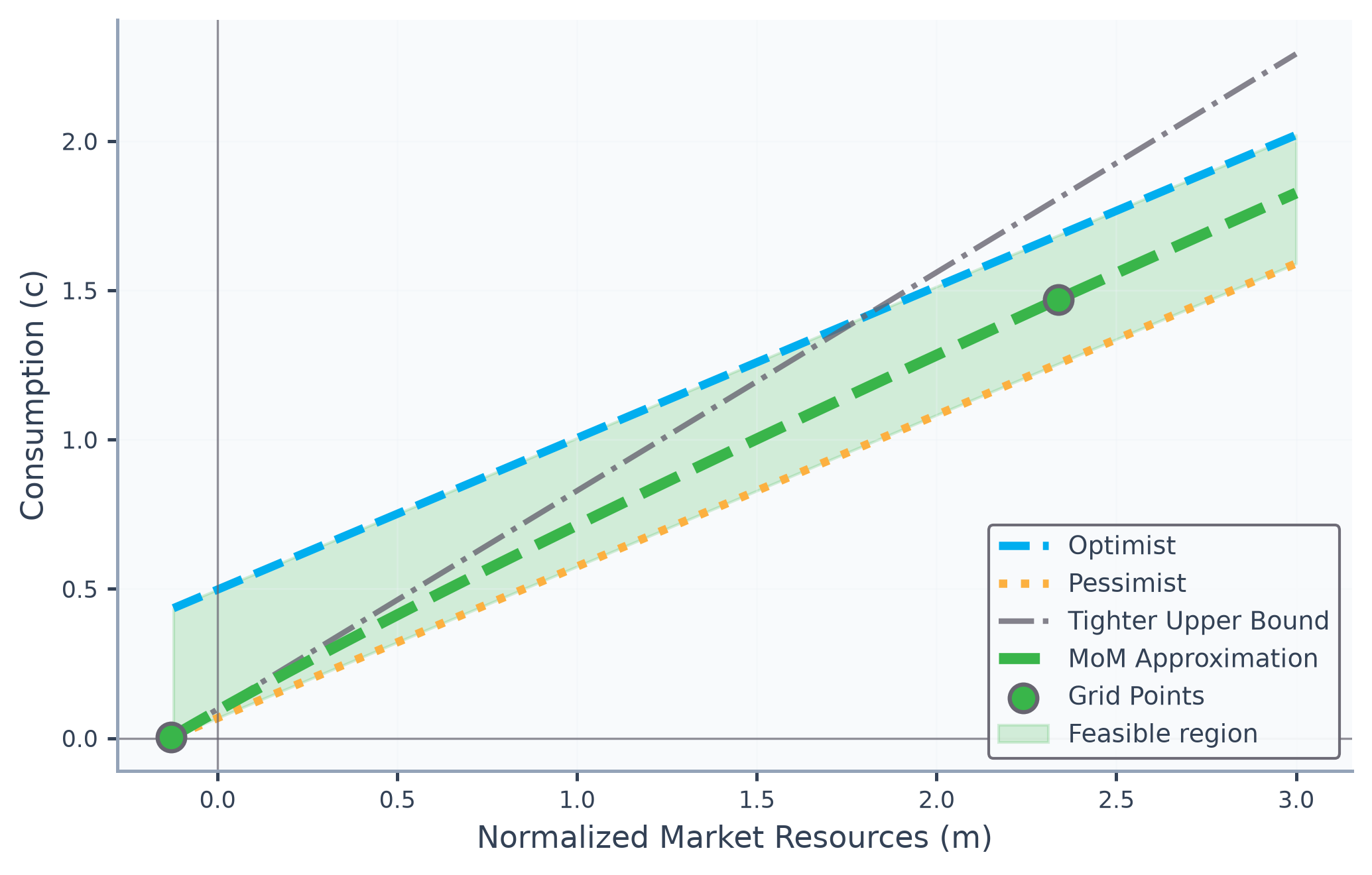
Figure 8:The Tighter Bound Binds Below the Cusp, the Optimist’s Bound Above It
6.2Hermite Interpolation
Although linear interpolation that matches the level of at the gridpoints is simple, Hermite interpolation Fritsch & Carlson, 1980Fritsch & Butland, 1984Hyman, 1983 matches both the level and the derivative of there. That derivative is supplied by the envelope condition Benveniste & Scheinkman, 1979Milgrom & Segal, 2002 together with the EGM Euler equation, so the interpolated rule matches, at each solved gridpoint, the marginal propensity to consume that the solution implies as well as the level.[15]
The slopes we need come from the moderation ratio itself. Since its argument is the log of excess market resources, the derivative measures how quickly the realist approaches the optimist as resources increase:
The interpolant carries the logit of (16) rather than itself, and the chain rule gives its derivative:
It turns out that this is all the slope data a cubic Hermite interpolant needs.[16] Differentiating (17) yields a moderation form for the MPC:[17]
where
Read the other way, this says we need no second approximation for the marginal propensity to consume. It is the derivative of the object we have already approximated, rescaled so that places the slope between and exactly as places the level between the pessimist and the optimist. Matching slopes as well as levels at each gridpoint therefore gives a consumption rule whose implied MPC agrees with the solved one at every node.
The pairing also explains why Figure 9 falls where Figure 3 climbs. The extra factor keeps the two from being mirror images. As levels off near one its derivative falls toward zero, and the factor falls with it.
At gridpoints the weight lies in by construction. Equation (37) rearranges to , and theory guarantees wherever the Euler equation is solved. Between gridpoints the property is not guaranteed, and we rely on the grid being fine enough to preserve it.
The weight reflects precautionary intensity, increasing when market resources are low relative to human wealth ( large) and when the moderation ratio responds sharply to changes in log excess resources ( large). As , and the MPC approaches the optimist’s minimal value ; as , and the MPC approaches the maximal value at the borrowing constraint.
Figure 9 shows both limits on the solved rule, with the moderated MPC inside the band at every solved gridpoint.
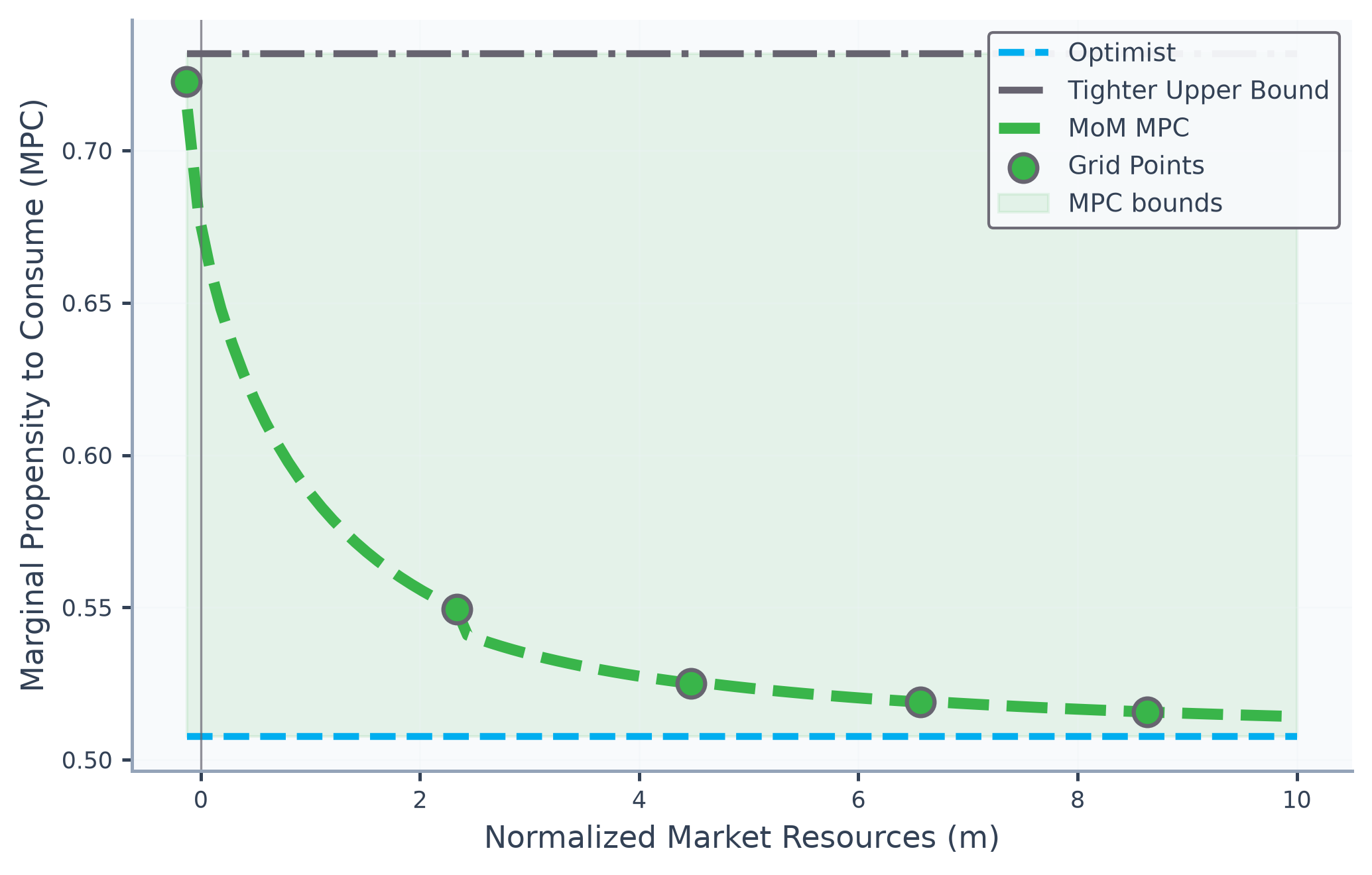
Figure 9:The Moderated MPC Is a Weighted Average of Its Two Limits at Every Solved Gridpoint
We now repeat the experiment of Table 1 in Table 2 with cubic Hermite in place of linear interpolation, for both methods on the same five-point grid.
Moderation’s interior errors fall by a factor of five in the first interval and by roughly two to three orders of magnitude in the rest. EGM improves too, but by less beyond the first interval, where moderation’s advantage grows from eleven or seventeen times under linear interpolation to between thirty-eight and fifty-six times under cubic, while in the first interval it slips from about three and a half times to three. The higher order gains more on the transformed moderation ratio than on consumption itself, so refining the interpolation widens the gap between the two methods.
Beyond the top gridpoint the errors barely move, 3.0(-3) to 2.4(-3) for moderation, and the ratio between the methods is forty-six in one table and forty-five in the other. Both moderation variants extrapolate the logit linearly there, so the beyond-grid advantage comes entirely from the change of variables, since interpolation order matters only where there are gridpoints to interpolate between.
The value function needs the same two ingredients, and we already have both in hand. Since is constant under perfect foresight, the optimist’s inverse value function has a constant slope with respect to cash-on-hand:
The derivative of the value moderation ratio (23) with respect to the log-gap argument is
where is given by (39) and is the derivative of the realist’s inverse value function. The pessimist’s inverse value function has the same derivative , since both are linear perfect foresight solutions.
We apply the same transformation to the value-based moderation ratio, which converts the bounded ratio into an unconstrained slope:
Note that , so the chain rule supplies their derivatives and nothing further need be solved for. The first derivative is:
The first- and second-derivative connections are:
If we also match the second derivative in (43) with a higher-order Hermite polynomial (with obtained by differentiating the expression for once more), the approximation matches the marginal propensity to consume at the gridpoints as well.[18]
6.3Artificial Borrowing Constraints
Nothing in (30) requires the borrowing constraint to be the natural one. A modeler who imposes a constraint tighter than the natural one changes both and , and we need change nothing else: when the artificial constraint binds, (the derivation behind (27) presumes the natural constraint; against an artificial one the consumer spends every unit above the floor) and the tighter bound is the budget line itself; when the constraint is natural, and the bound lies strictly inside it. One expression covers both cases, which is fortunate, because a modeler who has just tightened a constraint is rarely in the mood to rederive an approximation.
The two bounds always cross, so the question for us is whether our realist ever reaches the tighter one. Under a natural constraint they approach only as and touch it at the single point where both are zero, so the envelope has nothing to do. Under an artificial constraint they spend every resource they have over a whole interval above the constraint, up to the first kink point where it ceases to bind, and over that interval the envelope stops approximating and reproduces their rule.
Table 3:Maximum absolute consumption errors for as the artificial borrowing constraint tightens, EGM and MoM on the same five-point grid against a dense reference solution. is the period- value; the last column is the interval over which the realist’s rule coincides with the tighter bound.
| EGM | MoM | rule coincides with bound | ||
| natural | 0.732 | 5.4(-2) | 1.5(-2) | nowhere |
| -0.10 | 1.000 | 4.5(-2) | 6.9(-3) | |
| -0.05 | 1.000 | 3.4(-2) | 7.3(-3) | |
| 0.00 | 1.000 | 2.6(-2) | 7.5(-3) | |
| 0.10 | 1.000 | 1.6(-2) | 7.0(-3) |
We report what happens as we tighten the constraint in Table 3. The region over which the rule coincides with the bound grows, and moderation remains more accurate than endogenous gridpoints throughout. The advantage is largest where the constrained region is smallest, because that is where a method without the bound has the most room to overshoot it. We should be candid about how much rests on the envelope here. Drop it, and the moderated rule breaches the budget constraint in every row with an artificial constraint, spending resources the consumer does not have. The breach grows as the constraint tightens, and in the two tightest rows it is large enough to reverse the ordering (at the breach reaches 0.045, and the worst-case error of is now the larger of the two). Only the natural row, where the envelope has nothing to do, is unaffected.
6.4Assets as the State Variable
We have written the consumption problem in market resources, while the standard incomplete-markets models of Huggett (1993), Aiyagari (1994), and Krusell & Smith (1998) are written in assets and spend most of their computational budget solving the household problem we have been bracketing. Everything above transfers, because the bounds are perfect-foresight rules that hold at every , and is a function of whatever state the model uses.
To see that transfer, write down what those models actually carry. The state is the pair : assets carried into the period, which together with consumption determine next period’s assets as , and income , a finite Markov chain with transition matrix . Since , both bounds are affine in with the common slope :
The optimist’s human wealth is expected discounted income along the chain, and carries the state because the chain does, while the pessimist’s is the lowest income forever, the constant whose negative is the natural borrowing limit of Aiyagari (1994). Current income cancels from the gap, so the bracket has width , a quantity formed once per income state and constant in within it, which is all the moderation ratio requires. The transformation and interpolation above are unchanged, applied to within each income state.
The household problem transfers, though the layers above it do not, and on those (the fixed point in prices, the stationary distribution, the forecasting rule that closes a model with aggregate shocks) we say nothing.
7Risky Returns and Portfolio Choice
The variations so far all concern how the consumption rule is approximated, while the asset structure has stayed the same, one riskless asset earning a known . We now relax that in two steps, first making the return stochastic, so that the consumer’s savings are entirely invested in a risky asset, and then letting the fraction so invested be a choice.
The two problems without a portfolio choice are the corners of that choice, since holding the risky share at zero recovers the riskless model of the preceding sections, and holding it at one recovers the model of Section 7.1. Making the return risky changes the bounds of the consumption rule, since the limiting marginal propensity to consume is no longer -based, but it leaves the object being moderated where it was. Making the share a choice opens the interior between the corners and adds a second rule to approximate. Only the second step requires a new ingredient, because the transform that linearizes consumption does not linearize the share.
7.1Idiosyncratic Rate-of-Return Risk
Thus far we have assumed that the interest factor is constant at . Extending the previous derivations to allow for a perfectly forecastable time-varying interest factor would be trivial. Allowing for a stochastic interest factor is not trivial: it changes the two constants the bracket is built from, and , though nothing else. We treat return risk that is idiosyncratic, the return on a household-specific asset such as a private business or housing, drawn independently across households and over time Benhabib & Bisin, 2018, so the household’s problem acquires no aggregate state and the interest factor is i.i.d.,[19]
Both constants come from the high-wealth limit, where labor income is negligible relative to financial wealth, because in this case Merton (1969) and Samuelson (1969) showed that for a consumer without labor income the consumption function is linear, with an MPC that is the of the bracket,
positive under the stochastic-return impatience condition , the i.i.d.-return analogue of Carroll, 2020Benhabib & Bisin, 2018Chipeniuk et al., 2022. Human wealth needs a rate to discount at, and with no traded riskless asset there is none for us to appeal to, but the Euler equation supplies one, the implicit riskless return of the economy, which is the reciprocal of the expected stochastic discount factor Campbell & Viceira, 2002. In the same limit consumption grows at , so that discount factor is , and substituting (46) for cancels the preference parameters, leaving the shadow riskless return ,
so we obtain the two human wealths by writing their riskless expressions with in place of , and . The two constants use the return distribution differently, the MPC needing the single moment and human wealth the ratio of two, and a deterministic return collapses that ratio onto , which is why we needed only one rate when the return was certain. Finite human wealth requires , the return-risk counterpart of the finite-human-wealth condition (the riskless-return conditions are in Carroll & Shanker (2026)).
With the of (46) and the of (47) in place, the earlier construction applies unchanged. But the two sides of the bracket rest on different footing. Carroll & Lujan (2026) prove at full generality that the pessimist’s rule bounds optimal consumption from below whether or not returns are risky. The upper bound is open there, because the Jensen step that delivers it under deterministic returns fails once the return enters the marginal-utility argument. We check the upper bound numerically, and with the mean return equal to the riskless return of the earlier calibration and a level standard deviation of 0.08, the realist’s rule stays strictly inside the bracket at every one of two thousand evaluation points between the borrowing constraint and , the moderation ratio ranging over .[20]
7.2Portfolio Choice
Every application so far has moderated a consumption rule between two perfect-foresight consumption rules. The share of savings held in the risky asset is a sterner test, being a different choice variable with bounds of a different kind.
The share has a single limiting agent instead of two. As wealth grows, labor income becomes negligible and the optimal share approaches the constant that solves the portfolio problem of an investor with financial wealth alone Samuelson, 1969Merton, 1969, the first-order condition
This is a single-period problem, which is why Campbell & Viceira (2002) call its solution the ‘myopic’ share, and with i.i.d. returns it is the same at every wealth level. Their log-linear approximation gives 0.28 at the calibration below, whereas we use the 0.31 solved numerically on the discretized return process, for which it is exact. That limit is also a floor, because human wealth is a bond-like position, so that a household holding it tilts financial wealth toward the risky asset, and the share lies above at every finite wealth level Campbell & Viceira, 2002Viceira, 2001. That floor depends on income shocks being independent of returns, as they are here. When labor income is cointegrated with the stock market, the young want to short the market Benzoni et al., 2007, and is no floor at all.
The two characters of the consumption problem are of no use here. A pessimist who expected the worst return every period would hold no stock at all (the worst return is below the riskless one), and an optimist who ignored the risk would hold nothing else, so a bracket built on the pair would be the constraint set itself, within which moderating the share is the same thing as interpolating it. The upper edge is instead a constraint: the prohibition on borrowing to invest, . This is the upper half of the share constraint that the portfolio literature imposes alongside Cocco et al., 2005, as we do here. Together the two rule out debt of any kind, so next period’s resources are at least the income floor whatever the return turns out to be. They also supply a ceiling the share would otherwise not have, since a household with labor income to lean on would, if unconstrained, put an ever larger multiple of its financial wealth into the risky asset as that wealth shrank toward zero. We call the upper half the leverage constraint, to keep it distinct from the constraint on assets.
The bracket is therefore , and its width is constant in the state, as the width of the consumption bracket is. Bodie et al. (1992) obtain a tighter ceiling, , for riskless labor income, but the solved share crosses it here, because that ceiling’s gap above is proportional to , while the solved share’s gap closes more slowly. So we bracket against the constraint, which cannot be crossed.
The illustrations solve the infinite-horizon problem with relative risk aversion , discount factor 0.9, survival probability 0.98 (which scales the discount factor), riskless return , permanent income growth factor 1.01, permanent and transitory income shocks each with log standard deviation 0.1, a five percent chance of an unemployment draw paying thirty percent of permanent income, and a risky asset with mean gross return 1.08 and log standard deviation 0.184. The construction does not depend on these choices.
The moderation ratio for the share, , records where the solved share lies in its bracket, as does for consumption. The share approaches its limiting value only as wealth grows, so asymptotically and straightens that tail. Its other bound, the leverage constraint, is attained at finite wealth, where diverges, so the logit of Section 4.2 is the wrong transform here and the logarithm alone is the right one.
Figure 10 shows the consequence, with each candidate transformation rescaled to a common range and drawn against the straight chord through its own endpoints. Over the untransformed share departs from its chord by 39 percent of the plotted range and the logit by 14 percent, while departs by 1.4 percent. Scored on accuracy against a converged reference with five nodes, the logarithm is roughly a hundred times more accurate than interpolating the share itself, the complementary log-log, , eight times, and the logit four times. Nothing here fixes how the share approaches its limit, since the interpolant is fitted to the solved gridpoints, so a calibration whose tail behaves differently is served by the same construction.
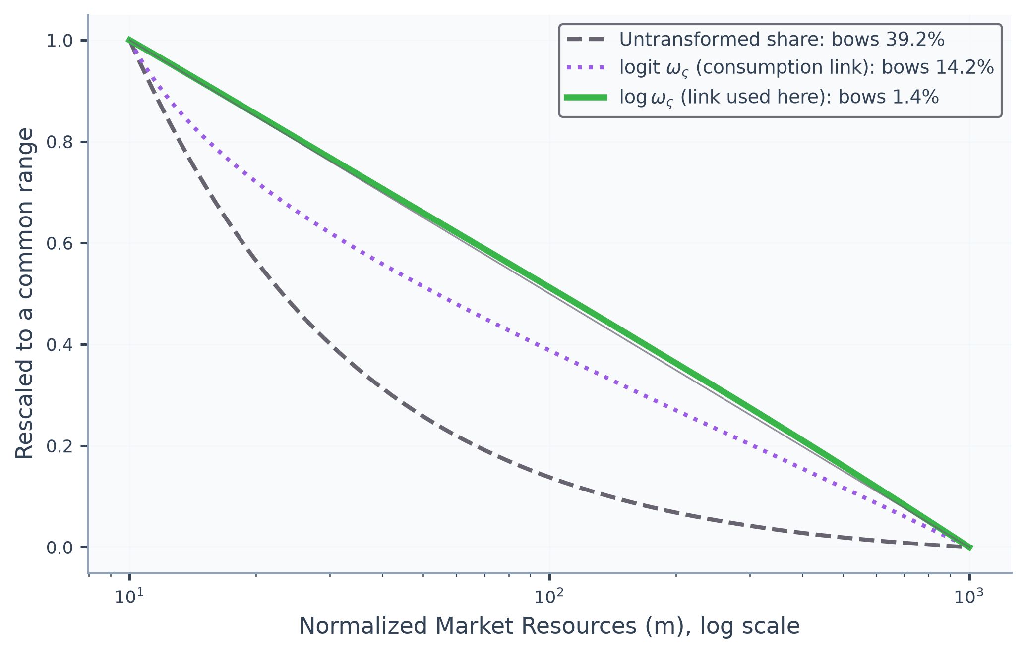
Figure 10:The Logarithm of the Share’s Moderation Ratio Is Nearly Straight Where the Logit Bows
At low wealth the leverage constraint binds and the solved share is exactly one. The point at which it stops binding is a kink in the share function, and unlike the cusp of (29) it has no closed form. The cusp was the intersection of two straight lines whose coefficients we knew, whereas the kink is the level of wealth at which the investor’s own first-order condition first holds with the share at one, and that depends on next period’s marginal value, which we do not know until the problem has been solved. So we take the kink from the solved rule, in which the investor leaves the constraint at (Figure 11). The approximation is exact on the constraint below it, moderated above it, and joined across it by a Hermite segment matched in level and slope at the two adjacent gridpoints. A cubic matched at both ends can overshoot the endpoint it starts from, so the approximation takes the lower envelope against the constraint, as the consumption rule does against , since the solved share never exceeds one.
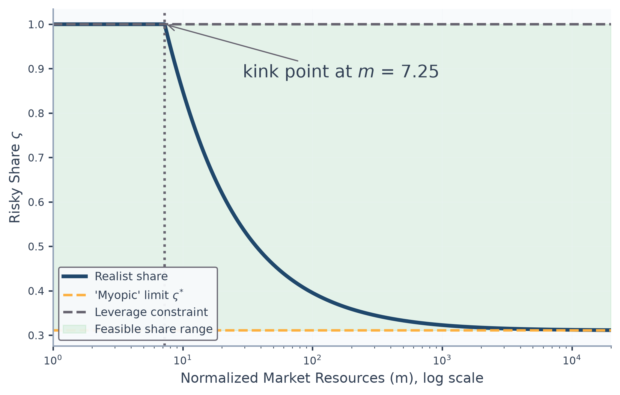
Figure 11:The Share Is Fully Invested Until Its Kink Point, Then Descends Toward Its Limit
Clear of the kink point, moderation is between seventy and a hundred and fifty times more accurate than interpolating the share directly on the same four to seven nodes, with the advantage growing as the grid coarsens. On a grid spanning the constrained region the advantage is smaller, and the reader is entitled to the whole picture. In the tail it runs from twelve to over a hundred times, across the transition it is about twice, and on a grid coarse enough that the kink point falls in a wide interval our joining segment is worse than plain interpolation there.
Beyond the top gridpoint, Figure 12 is the portfolio analogue of Figure 1. Linear extrapolation carries the share below its limiting value, a portfolio no optimizing investor would hold at any wealth, while the moderated rule continues the descent recorded at the solved gridpoints and approaches the limit from above.
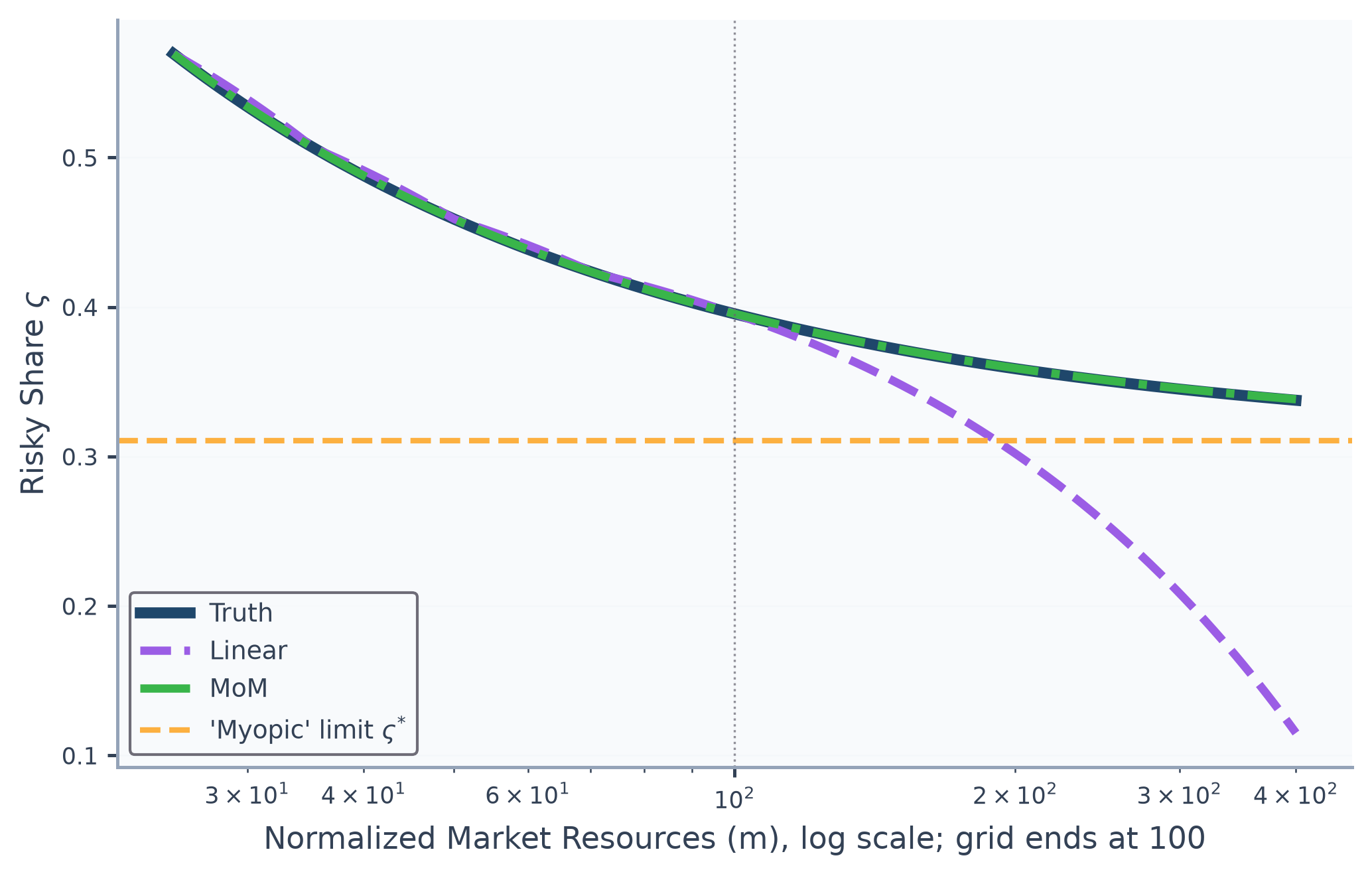
Figure 12:Beyond the Grid, Linear Extrapolation Breaches the Limiting Share and Moderation Does Not
Before we claim too much, we should say that the share is an output of each period’s optimization rather than an input to the next period’s, so a moderated share does not propagate through the backward induction the way a moderated consumption rule does. The construction supplies a representation, one in which the expensive per-node optimization can be performed on far fewer nodes because the share between them is moderated instead of interpolated.
8Conclusion
The method proposed here is not universally applicable. For example, the method cannot be used for problems for which upper and lower bounds to the ‘true’ solution are not known. Those bounds need not come in pairs of perfect-foresight agents, as the portfolio application shows by bracketing the share between the ‘myopic’ investor and the leverage constraint. But many problems do have obvious upper and lower bounds, and in those cases (as in the consumption and portfolio examples used in the paper), the method may result in substantial improvements in accuracy and stability of solutions.
Acknowledgments
We thank Matthew N. White for many thoughtful conversations about the ideas in this paper. The views presented here are those of the authors and should not be attributed to the Japanese Ministry of Finance, the Reserve Bank of New Zealand, or Fannie Mae.
An early version of the paper was presented at the 2012 Society for Economic Dynamics meetings by Wu, Tokuoka, and Carroll, and Carroll (2020) discusses the method in lecture-note form. This paper supersedes both accounts.
The permanent-transitory decomposition is Friedman (1957); the stochastic process form is Muth (1960).
Bounded support () gives the consumption function well-defined upper and lower bounds. Results for unbounded shocks with finite moments (lognormal, for example) exist, and we do not pursue that extension.
We assume throughout, because the transformations of the value function below (, ) divide by . Log utility needs parallel derivations, with the same economics.
Restoring permanent shocks (a five-point discretization at standard deviation 0.1) moves every error reported below by less than a factor of two, on that calibration’s own endogenous gridpoints, and leaves the ordering of the two methods intact. The replication package’s verification script carries the switch.
The
HARKtoolkit does not (yet) extend the last linear segment, and instead shrinks the gap above the top gridpoint to the perfect-foresight limit exponentially, which keeps precautionary saving positive. That is the easy and obvious choice, the one we made early in the toolkit’s development, when the limiting bounds were known but the theory behind the approach to them was not yet worked out. It is also not how the true gap closes, and nothing in the calibration says how it should, so the accuracy it delivers at any wealth level is not knowable in advance. We therefore compare against linear extrapolation, which is the generic practice, whereas the method below takes its tail from the solved gridpoints.For a derivation, see Carroll & Shanker (2026); is defined therein as the MPC of the perfect foresight consumer with horizon .
Here denotes excess above minimum, not a time difference.
Under the GIC the limiting slope exists. It may equal zero in theory, but the boundary slope on any finite grid is strictly positive, and the bounds are preserved whichever slope is used.
Under perfect foresight, consumption grows at rate : . Discounting yields , so (unchanged for normalized variables). In the infinite-horizon limit, we write simply .
The replication package regenerates the tables and the numbers quoted in this section and checks each accuracy claim against the code.
The envelope also fixes behavior at the constraint itself, since vanishes at . Under an artificial constraint , EGM cannot place a gridpoint below the kink, because inverting the Euler equation from an asset grid gives with , so the smallest it reaches is , the kink itself, and no refinement of the grid creates gridpoints in a region that has no interior solution to invert.
Approximation quality between gridpoints is what ultimately limits any such method. Santos (2000) gauges it through Euler-equation residuals, as the lower panel of Table 1 does, and Judd et al. (2017) derives lower bounds on the resulting approximation errors.
Cubic Hermite interpolation of the transformed ratio takes node values from the transformation and node slopes . A monotone scheme Boor, 2001 (Fritsch-Carlson or Fritsch-Butland) treats those slopes as targets and adjusts them to enforce monotonicity.
The consumption function generated from the value function would then match both the level of consumption and the marginal propensity to consume at the gridpoints; within the grid, its numerical differences from the one constructed earlier are negligible.
Here is the log of the earlier calibration’s riskless return and the premium of the mean log return over it. Since no riskless asset trades in this subsection, the pair only parameterizes the distribution in the earlier units. The term makes , so raising is a mean-preserving spread of the level return, and the lognormal moment generating function gives , the expression the code evaluates.
The test suite asserts strict containment, not containment to a tolerance, and first checks that the spread lies below the volatility (near 0.10 here) at which overtakes , so that the condition above holds.
- Ma, Q., & Toda, A. A. (2022). Asymptotic Linearity of Consumption Functions and Computational Efficiency. Journal of Mathematical Economics, 98, 102562. 10.1016/j.jmateco.2021.102562
- White, M. N. (2015). The Method of Endogenous Gridpoints in Theory and Practice. Journal of Economic Dynamics and Control, 60, 26–41. 10.1016/j.jedc.2015.08.001
- Leland, H. E. (1968). Saving and Uncertainty: The Precautionary Demand for Saving. Quarterly Journal of Economics, 82(3), 465–473. 10.2307/1879518
- Sandmo, A. (1970). The Effect of Uncertainty on Saving Decisions. Review of Economic Studies, 37(3), 353–360. 10.2307/2296725
- Kimball, M. S. (1990). Precautionary Saving in the Small and in the Large. Econometrica, 58(1), 53–73. 10.2307/2938334
- Stachurski, J., & Toda, A. A. (2019). An Impossibility Theorem for Wealth in Heterogeneous-Agent Models with Limited Heterogeneity. Journal of Economic Theory, 182, 1–24. 10.1016/j.jet.2019.04.001
- Ma, Q., Stachurski, J., & Toda, A. A. (2020). The Income Fluctuation Problem and the Evolution of Wealth. Journal of Economic Theory, 187, 105003. 10.1016/j.jet.2020.105003
- Carroll, C. D. (2009). Precautionary Saving and the Marginal Propensity to Consume Out of Permanent Income. Journal of Monetary Economics, 56(6), 780–790. 10.1016/j.jmoneco.2009.06.016
- Ma, Q., & Toda, A. A. (2021). A Theory of the Saving Rate of the Rich. Journal of Economic Theory, 192, 105193. 10.1016/j.jet.2021.105193
- Carroll, C. D. (1997). Buffer-Stock Saving and the Life Cycle/Permanent Income Hypothesis. Quarterly Journal of Economics, 112(1), 1–55. 10.1162/003355397555109
- Carroll, C. D., & Shanker, A. (2026). Theoretical Foundations of Buffer Stock Saving. Johns Hopkins University. https://llorracc.github.io/BufferStockTheory/BufferStockTheory.pdf
- Carroll, C. D. (2020). Solving microeconomic dynamic stochastic optimization problems [Techreport]. Johns Hopkins University. https://www.econ2.jhu.edu/people/ccarroll/SolvingMicroDSOPs.pdf
- Carroll, C. D. (2006). The method of endogenous gridpoints for solving dynamic stochastic optimization problems. Economics Letters, 91(3), 312–320. 10.1016/j.econlet.2005.09.013
- Barillas, F., & Fernández-Villaverde, J. (2007). A Generalization of the Endogenous Grid Method. Journal of Economic Dynamics and Control, 31(8), 2698–2712. 10.1016/j.jedc.2006.08.005
- Hintermaier, T., & Koeniger, W. (2010). The Method of Endogenous Gridpoints with Occasionally Binding Constraints among Endogenous Variables. Journal of Economic Dynamics and Control, 34(10), 2074–2088. 10.1016/j.jedc.2010.05.002