Appendix to "The Method of Moderation"
Abstract
This appendix provides detailed mathematical derivations and technical results supporting the Method of Moderation. Topics include: value function transformations and their relationship to the inverse value function; explicit formulas for minimal and maximal marginal propensities to consume; cusp point calculations for tighter upper bounds; Hermite interpolation slope formulas and MPC derivations; patience conditions ensuring well-defined solutions; and extensions to stochastic returns with explicit formulas for consumption problems with an exogenous risky return.
Patience Conditions Details
Each patience condition from the main text controls a distinct way the problem could misbehave. The FVAC guarantees that even autarky, saving nothing and consuming income as it arrives, delivers finite expected discounted utility, so the consumer has a reason to value resources at all. The AIC rules out indefinite deferral of consumption: under certainty the marginal utility of consuming now exceeds the discounted marginal utility of consuming later. Two further conditions bound wealth from opposite directions. The RIC holds asset growth below the patience-adjusted discount rate, so wealth cannot explode; the GIC holds consumption growth below permanent-income growth, which is what pins down a finite target wealth ratio. Finally, the FHWC keeps the present value of future labor income finite. Where these conditions fail, behavior changes qualitatively: when all hold, the consumer runs a buffer stock around a target wealth ratio; when the AIC fails, consumption grows without bound; when the GIC fails but the RIC still holds, wealth grows without bound Carroll, 1997Carroll, 2020Carroll & Shanker, 2024.
Human Wealth Formulas
The optimist’s human wealth (assuming ) can be computed three ways: backward recursion , ; forward sum ; or infinite-horizon when . With , .
The pessimist’s human wealth (assuming ) follows similarly: backward recursion , ; forward sum ; or infinite-horizon . When (unemployment), .
Marginal Propensity to Consume Formulas
The minimal MPC (perfect foresight consumer with horizon ) has three forms Carroll, 2009: backward recursion with ; forward sum ; or infinite-horizon .
The maximal MPC Carroll & Toche, 2009 satisfies backward recursion with ; forward sum ; or infinite-horizon .
A Tighter Upper Bound
The method in the main text does not guarantee that the approximation respects , where is the MPC at the natural borrowing constraint; near the constraint the optimist’s bound is loose because it is calibrated to the low MPC that prevails at high wealth. Carroll & Shanker (2024) derives the maximal MPC , where is the unemployment probability of Carroll & Toche (2009), extending the limiting-MPC formulas of Ma & Toda (2021). Strict concavity implies for low wealth, while the optimist’s bound is tighter for high wealth.
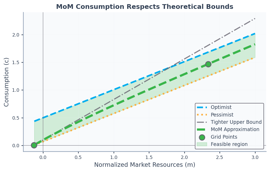
As Figure 1 shows, the two upper bounds intersect at the cusp point where
where since . For , the tighter upper bound yields
This motivates the low-resource moderation ratio, defined for as
Since , the right-hand side equals , which lies in for : the lower bound is the minimal MPC and the upper bound is the maximal MPC , with strict inequality at the upper end following from . Applying the logit transformation and interpolating as before yields consumption satisfying both upper bounds throughout. For computational robustness we combine the pieces into a three-part approximation: the tighter bound below the cusp, the optimist’s bound above, and a Hermite segment (below) bridging the cusp, where the two bounds meet at equal levels but different slopes. Because the Hermite segment is matched to the level and the slope of the adjacent piece at each of its endpoints, the combined consumption function is continuous and differentiable and respects all theoretical constraints.
Value Function Derivation
Under perfect foresight, consumption grows at constant rate equal to the absolute patience factor : . The present discounted value of consumption, discounting the stream at the return , satisfies . Dividing by consumption yields the PDV-to-consumption ratio , which is unchanged for normalized variables. Defining , this yields the key identity , connecting the infinite-horizon PDV-to-consumption ratio to the minimal MPC.
The optimist’s value function satisfies
The infinite horizon expression becomes
This can be transformed as
The transformation is the inverse utility ; for log utility () it becomes , the limit, so the construction carries over to log utility unchanged.
The pessimist’s inverse value follows by the same steps, with :
so that , the denominator that normalizes the value moderation ratio below.
For the realist’s problem, we define . At each the values are ordered : the realist’s true income process stochastically dominates the pessimist’s worst-case income and is dominated, for a risk-averse agent, by the optimist’s certain expected income. Because the inverse-value transform is monotonic, the same ordering holds for , and we define
and the logit-transformed counterpart:
Inverting these approximations yields
from which the value function approximation is .
Hermite Interpolation
The numerical accuracy of the method of moderation depends critically on the quality of function approximation between gridpoints Santos, 2000. Our bracketing approach complements work that bounds numerical errors in dynamic economic models Judd et al., 2017. Although linear interpolation that matches the level of at the gridpoints is simple, Hermite interpolation Fritsch & Carlson, 1980 offers a considerable advantage.
The moderation ratio derivative measures how quickly the realist approaches the optimist as resources increase. Differentiating (11) with respect to we obtain
Rearranging this yields a moderation form for the marginal propensity to consume:
where
Carroll & Shanker (2024) guarantees at gridpoints where the Euler equation holds, so and the expression above is indeed a convex combination of and . At very high wealth, and the MPC approaches ; near the borrowing constraint, and the MPC approaches .
For Hermite interpolation, compute at gridpoints, then derive for slope data. By matching both the level and the derivative of at the gridpoints, where the derivative is obtained from the envelope condition Benveniste & Scheinkman, 1979Milgrom & Segal, 2002 together with the EGM Euler equation, the interpolated consumption rule satisfies the Euler equation exactly at each solved gridpoint. These techniques extend naturally to the value function approximation.
For monotone cubic Hermite schemes Fritsch & Carlson, 1980Fritsch & Butland, 1984Boor, 2001, theoretical slopes may be adjusted to enforce monotonicity Hyman, 1983. The Fritsch-Carlson algorithm modifies slopes at local extrema, while Fritsch-Butland uses harmonic mean weighting. Both preserve the shape-preserving property essential for consumption functions that must be strictly increasing.
Stochastic Rate of Return
For i.i.d. returns with ,[1] Samuelson (1969)Merton (1969)Merton (1971) showed that for a consumer without labor income (or with perfectly forecastable labor income) the consumption function is linear, with an MPC , which is positive under the stochastic return impatience condition (the i.i.d.-return analogue of the RIC ). See Carroll (2020)Benhabib & Bisin (2018)Chipeniuk et al. (2021) for extensions. The pessimist and the optimist face certain income but the same stochastic return, so the Merton-Samuelson result applies to both and their consumption functions remain linear. The realist faces both labor income and return risk, and the moderation ratio captures their combined precautionary response. In this case the previous analysis applies once we substitute this MPC for the one that characterizes the perfect-foresight problem without rate-of-return risk. As Figure 2 shows, consumption remains bounded between the pessimist and the optimist, each of which (for ) consumes slightly less in the face of return uncertainty; for the effect reverses.
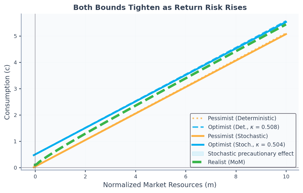
Figure 2:Effect of Return Uncertainty on Consumption Bounds
The fact that a linear consumption function with an MPC satisfies the Euler equation with i.i.d. returns and no labor income can be derived by the method of undetermined coefficients. In particular, assume that , with a time-independent MPC to be determined. Substituting this into the Euler equation, we have
where the second equality uses the assumed form of the consumption function. Since there is no labor income, . Substituting this into the above we obtain
Solving for and recalling that returns are i.i.d. gives .
In the particular case of lognormal returns, the MPC can be written in closed form. The moment generating function (MGF) of the normal variable provides the key formula. For , the MGF is . Setting and yields[2]
Simplifying the variance terms: , giving the final form
Here is the log risk-free rate and is the equity premium (the expected excess log return). This parametrization ensures , so that increasing constitutes a mean-preserving spread of the level of the return.
Here we can interpret as the risk premium, that is, the additional average return from holding a risky asset compared to the risk-free rate . Adjusting the average log return by the asset volatility ensures that increasing constitutes a mean-preserving spread of the level of return.
- Carroll, C. D. (1997). Buffer-Stock Saving and the Life Cycle/Permanent Income Hypothesis. Quarterly Journal of Economics, 112(1), 1–55. 10.1162/003355397555109
- Carroll, C. D. (2020). Solving microeconomic dynamic stochastic optimization problems [Techreport]. Johns Hopkins University. https://www.econ2.jhu.edu/people/ccarroll/SolvingMicroDSOPs.pdf
- Carroll, C. D., & Shanker, A. (2024). Theoretical Foundations of Buffer Stock Saving (Revise and Resubmit, Quantitative Economics). Johns Hopkins University. https://llorracc.github.io/BufferStockTheory/BufferStockTheory.pdf
- Carroll, C. D. (2009). Precautionary Saving and the Marginal Propensity to Consume Out of Permanent Income. Journal of Monetary Economics, 56(6), 780–790. 10.1016/j.jmoneco.2009.06.016
- Carroll, C. D., & Toche, P. (2009). A Tractable Model of Buffer Stock Saving (Working Paper No. 15265). National Bureau of Economic Research. 10.3386/w15265
- Ma, Q., & Toda, A. A. (2021). A Theory of the Saving Rate of the Rich. Journal of Economic Theory, 192, 105193. 10.1016/j.jet.2021.105193
- Santos, M. S. (2000). Accuracy of Numerical Solutions Using the Euler Equation Residuals. Econometrica, 68(6), 1377–1402. 10.1111/1468-0262.00165
- Judd, K. L., Maliar, L., & Maliar, S. (2017). Lower Bounds on Approximation Errors to Numerical Solutions of Dynamic Economic Models. Econometrica, 85(3), 991–1020. 10.3982/ecta12791
- Fritsch, F. N., & Carlson, R. E. (1980). Monotone Piecewise Cubic Interpolation. SIAM Journal on Numerical Analysis, 17(2), 238–246. 10.1137/0717021
- Benveniste, L. M., & Scheinkman, J. A. (1979). On the Differentiability of the Value Function in Dynamic Models of Economics. Econometrica, 47(3), 727–732. 10.2307/1910417
- Milgrom, P., & Segal, I. (2002). Envelope Theorems for Arbitrary Choice Sets. Econometrica, 70(2), 583–601. 10.1111/1468-0262.00296
- Fritsch, F. N., & Butland, J. (1984). A Method for Constructing Local Monotone Piecewise Cubic Interpolants. SIAM Journal on Scientific and Statistical Computing, 5(2), 300–304. 10.1137/0905021
- de Boor, C. (2001). A Practical Guide to Splines (Revised, Vol. 27). Springer. 10.1007/978-1-4612-6333-3
- Hyman, J. M. (1983). Accurate Monotonicity-Preserving Cubic Interpolation. SIAM Journal on Scientific and Statistical Computing, 4(4), 645–654. 10.1137/0904045
- Samuelson, P. A. (1969). Lifetime Portfolio Selection by Dynamic Stochastic Programming. Review of Economics and Statistics, 51(3), 239–246. 10.2307/1926559