The Method of Moderation: Illustrative Notebook

---
# MyST frontmatter (inherits authors, bibliography from myst.yml)
title: Illustrative Notebook
short_title: Notebook
description: A pedagogical introduction to the Method of Moderation with interactive code examples.
# Jupytext configuration
---

The Method of Moderation: Illustrative Notebook¶

# Import Econ-ARK styling and display header
from style import (
    HEADER_HTML_NOTEBOOK,
    apply_ark_style,
    apply_notebook_css,
)

# Apply Econ-ARK branding and styling
apply_ark_style()
apply_notebook_css()


# Display Econ-ARK header (for Jupyter notebooks)
from IPython.display import HTML, display

display(HTML(HEADER_HTML_NOTEBOOK))

Author: Alan Lujan, Johns Hopkins University

This notebook provides a pedagogical introduction to the Method of Moderation (MoM), a novel technique for solving consumption-saving models with superior accuracy and stability. We begin by motivating the problem that MoM solves: the “extrapolation problem” inherent in sparse-grid implementations of the Endogenous Grid Method (EGM). We then build the theoretical foundations for MoM, demonstrating how it leverages analytical bounds to ensure economically sensible behavior across the entire state space.

Model Foundations: The Friedman-Muth Income Process¶

We adopt the canonical framework of Friedman (1957) and Muth (1960): an agent receiving labor income subject to permanent and transitory shocks. The model implementation follows Carroll (2020).

The Extrapolation Problem in Consumption-Saving Models¶

The Method of Moderation (MoM) addresses the extrapolation problem in sparse-grid EGM implementations. EGM computes optimal consumption at finite grid points, but evaluating the policy function outside this grid via linear extrapolation can predict negative precautionary saving, violating established theory Leland, 1968Sandmo, 1970Kimball, 1990.

MoM operates in a transformed space defined by two analytical bounds from the buffer-stock saving literature Carroll, 1997Stachurski & Toda, 2019Ma et al., 2020:

The Optimist: Ignores future income risk.
The Pessimist: Assumes worst-case income realizations.

The true consumption function lies between these extremes. MoM interpolates a moderation ratio guaranteed to remain within bounds, producing solutions that are economically coherent across the entire state space.

from __future__ import annotations

from moderation import (
    IndShockEGMConsumerType,
    IndShockMoMConsumerType,
    IndShockMoMStochasticRConsumerType,
)
from plotting import (
    GridType,
    plot_consumption_bounds,
    plot_cusp_point,
    plot_logit_function,
    plot_moderation_ratio,
    plot_mom_mpc,
    plot_precautionary_gaps,
    plot_stochastic_bounds,
    plot_value_functions,
)

# Model setup: Consumer with income uncertainty
params = {
    "CRRA": 2.0,
    "DiscFac": 0.96,
    "Rfree": [1.02],
    "TranShkStd": [1.0],
    "cycles": 1,
    "LivPrb": [1.0],
    "vFuncBool": True,
    "CubicBool": True,
    "PermGroFac": [1.0],
    "PermShkStd": [0.0],
    "TranShkCount": 7,
    "UnempPrb": 0.0,
    "BoroCnstArt": None,
}

# Dense grid for "truth" solution (high precision)
dense_grid = {"aXtraMin": 0.001, "aXtraMax": 40, "aXtraCount": 500, "aXtraNestFac": 3}

# Sparse grid for practical comparison (5 points only)
sparse_grid = {"aXtraMin": 0.001, "aXtraMax": 4, "aXtraCount": 5, "aXtraNestFac": -1}

# Solve three versions: Truth (dense EGM), Sparse EGM, Sparse MoM
IndShockTruth = IndShockEGMConsumerType(**(params | dense_grid))
IndShockTruth.solve()
IndShockTruthSol = IndShockTruth.solution[0]

# Unpack theoretical bounds (same for all methods)
TruthOpt = IndShockTruthSol.Optimist
TruthPes = IndShockTruthSol.Pessimist
TruthTight = IndShockTruthSol.TighterUpperBound

# Sparse EGM solution (standard approach)
IndShockEGMApprox = IndShockEGMConsumerType(**(params | sparse_grid))
IndShockEGMApprox.solve()
IndShockEGMApproxSol = IndShockEGMApprox.solution[0]

# Sparse MoM solution (same grid, different method)
IndShockMoMApprox = IndShockMoMConsumerType(**(params | sparse_grid))
IndShockMoMApprox.solve()
IndShockMoMApproxSol = IndShockMoMApprox.solution[0]

# Grid parameters for plotting
mNrmMax = IndShockMoMApproxSol.mNrmMin + IndShockMoMApprox.aXtraGrid.max()

Consumption Function Analysis¶

The first set of figures will focus on the core of the consumption-saving problem: the consumption function $\cFunc(\mNrm)$ , which maps market resources $\mNrm$ to consumption. We will demonstrate the extrapolation problem inherent in the standard EGM and show how the Method of Moderation resolves it by respecting theoretical bounds.

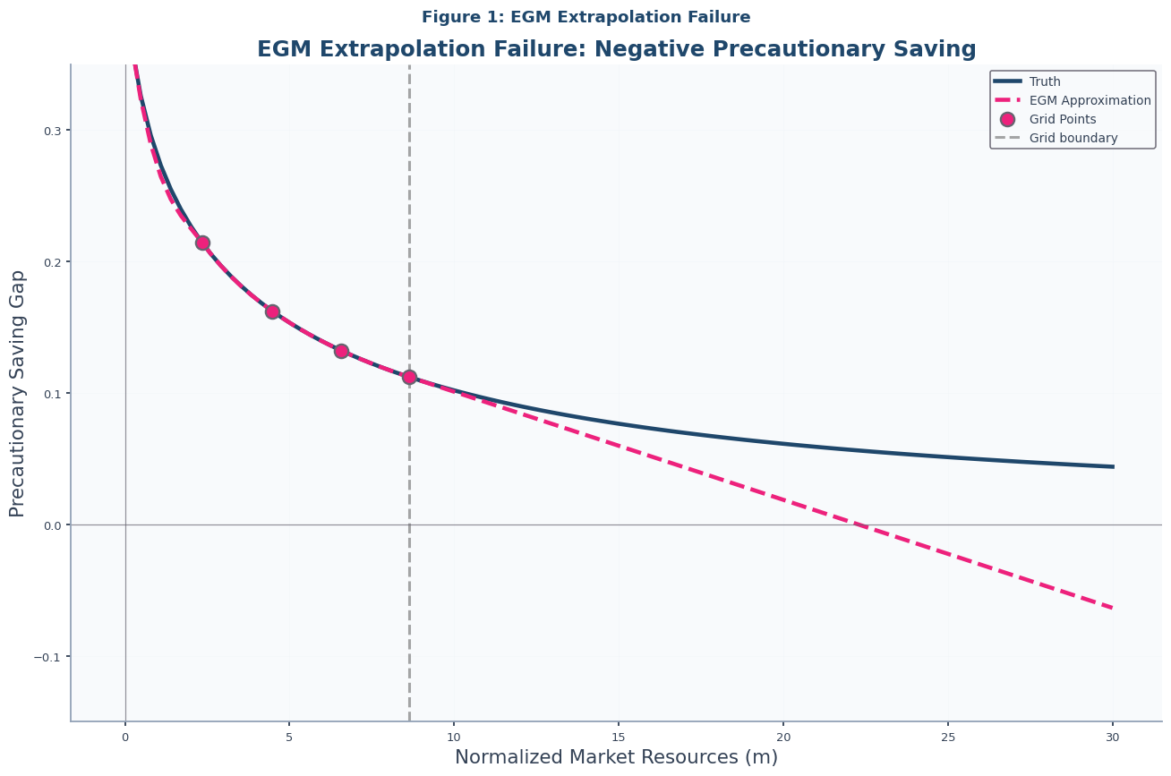
Figure 1: The EGM Extrapolation Problem¶

The precautionary saving gap (optimist minus realist consumption) must be positive: income risk induces additional saving. As demonstrated in the paper and shown in Notebook-code, standard EGM violates this constraint when extrapolating Carroll, 2006.

# Figure 1: EGM Extrapolation Failure
plot_precautionary_gaps(
    truth_solution=IndShockTruthSol,
    approx_solutions=IndShockEGMApproxSol,
    title="Figure 1: EGM Extrapolation Failure",
    subtitle="EGM Extrapolation Failure: Negative Precautionary Saving",
)

EGM in the Literature

The Endogenous Grid Method (Carroll (2006)) is a powerful and widely-used tool in computational economics. Its applications have been extended to solve multi-dimensional problems Barillas & Fernández-Villaverde, 2007, models with occasionally binding constraints Hintermaier & Koeniger, 2010, non-smooth and non-concave problems Fella, 2014, and discrete-continuous choice models Iskhakov et al., 2017. For a comprehensive treatment of the theory and practice of EGM, see White, 2015.

A critical step in implementing any numerical solution is the discretization of continuous stochastic processes. Standard methods for discretizing income shocks include those proposed by Tauchen & Hussey, 1991 and Tauchen, 1986.

Figure 2: Truth Bounded by Theory¶

The optimal consumption function is bounded by analytical optimist and pessimist solutions. Notebook-code (Figure 2 in the paper) confirms the high-precision “truth” lies between these bounds.

# Figure 2: Truth Bounded by Theory
plot_consumption_bounds(
    solution=IndShockTruthSol,
    title="Figure 2: Truth Bounded by Economic Theory",
    subtitle="True Consumption Always Lies Between Theoretical Bounds",
    show_grid_points=False,  # Truth solution has too many grid points to display clearly
)

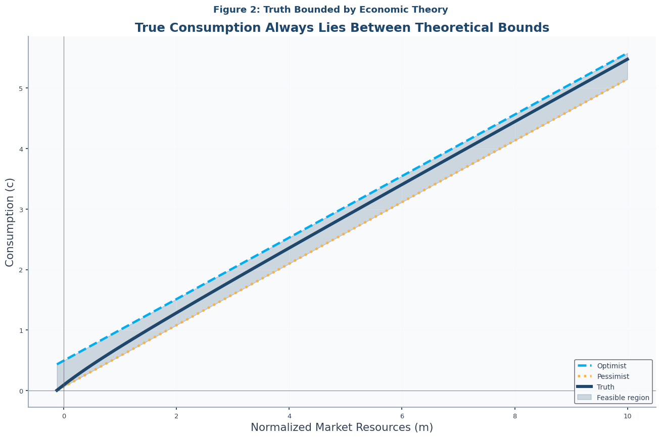
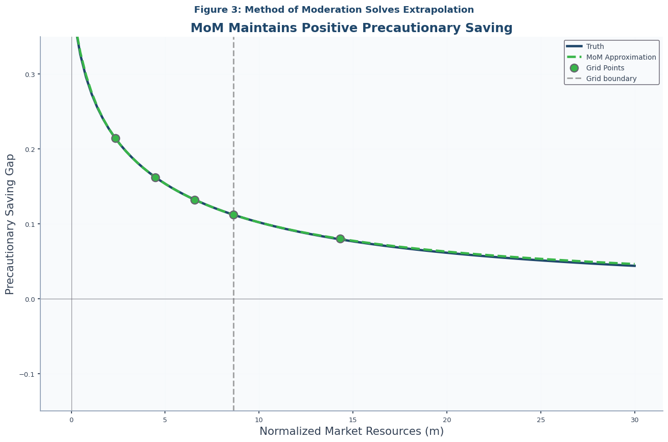
Figure 3: Method of Moderation Solution¶

MoM interpolates a moderation ratio in a transformed space that guarantees bound compliance. Notebook-code (Figure 3 in the paper) shows MoM maintains positive precautionary saving even far beyond the computed grid.

# Figure 3: Method of Moderation Success
plot_precautionary_gaps(
    truth_solution=IndShockTruthSol,
    approx_solutions=IndShockMoMApproxSol,
    title="Figure 3: Method of Moderation Solves Extrapolation",
    subtitle="MoM Maintains Positive Precautionary Saving",
)

MoM builds on EGM’s computational efficiency while enforcing theoretical bounds. See the paper’s algorithm.

MoM Algorithm Details

MoM steps (notation matches the paper):

Solve standard EGM for realist consumption at gridpoints
Transform to $\logmNrmEx = \log(\mNrm - \mNrmMin)$
Compute $\modRte(\logmNrmEx) = (\cFuncReal - \cFuncPes)/(\cFuncOpt - \cFuncPes) \in [0,1]$ (Eq. (9))
Apply logit: $\logitModRte = \log(\modRte/(1-\modRte))$
Interpolate $\logitModRte(\logmNrmEx)$ with derivatives
Reconstruct: $\cFuncReal = \cFuncPes + \modRte \cdot (\cFuncOpt - \cFuncPes)$

This ensures bound compliance via asymptotically linear extrapolation, as derived in the paper. HARK uses cubic Hermite interpolation Fritsch & Carlson, 1980Fritsch & Butland, 1984 for accuracy; see Santos, 2000Judd et al., 2017 on function approximation and error bounding.

Figure 4: MoM Consumption Function¶

Notebook-code (Figure 4 in the paper) shows MoM consumption between optimist and pessimist bounds, plus a tighter upper bound derived from $\MPCmax$ near the borrowing constraint Carroll, 2001Ma & Toda, 2021Carroll & Toche, 2009. The cusp intersection is given by (12).

# Figure 4: MoM Consumption Function
plot_consumption_bounds(
    solution=IndShockMoMApproxSol,
    title="Figure 4: MoM Consumption Function",
    subtitle="MoM Consumption Respects Theoretical Bounds",
    m_max=3.0,
    show_tight_bound=True,
)

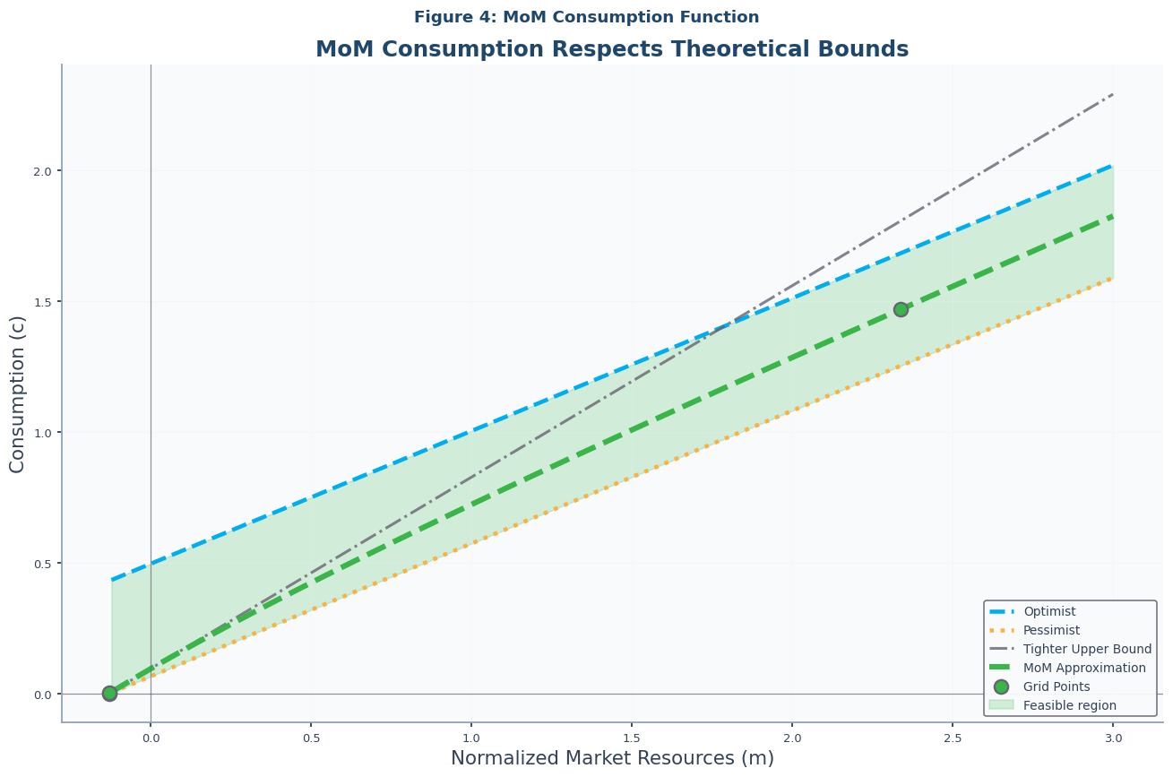
Bound Preservation: MoM consumption stays within theoretical bounds and below tight bound.

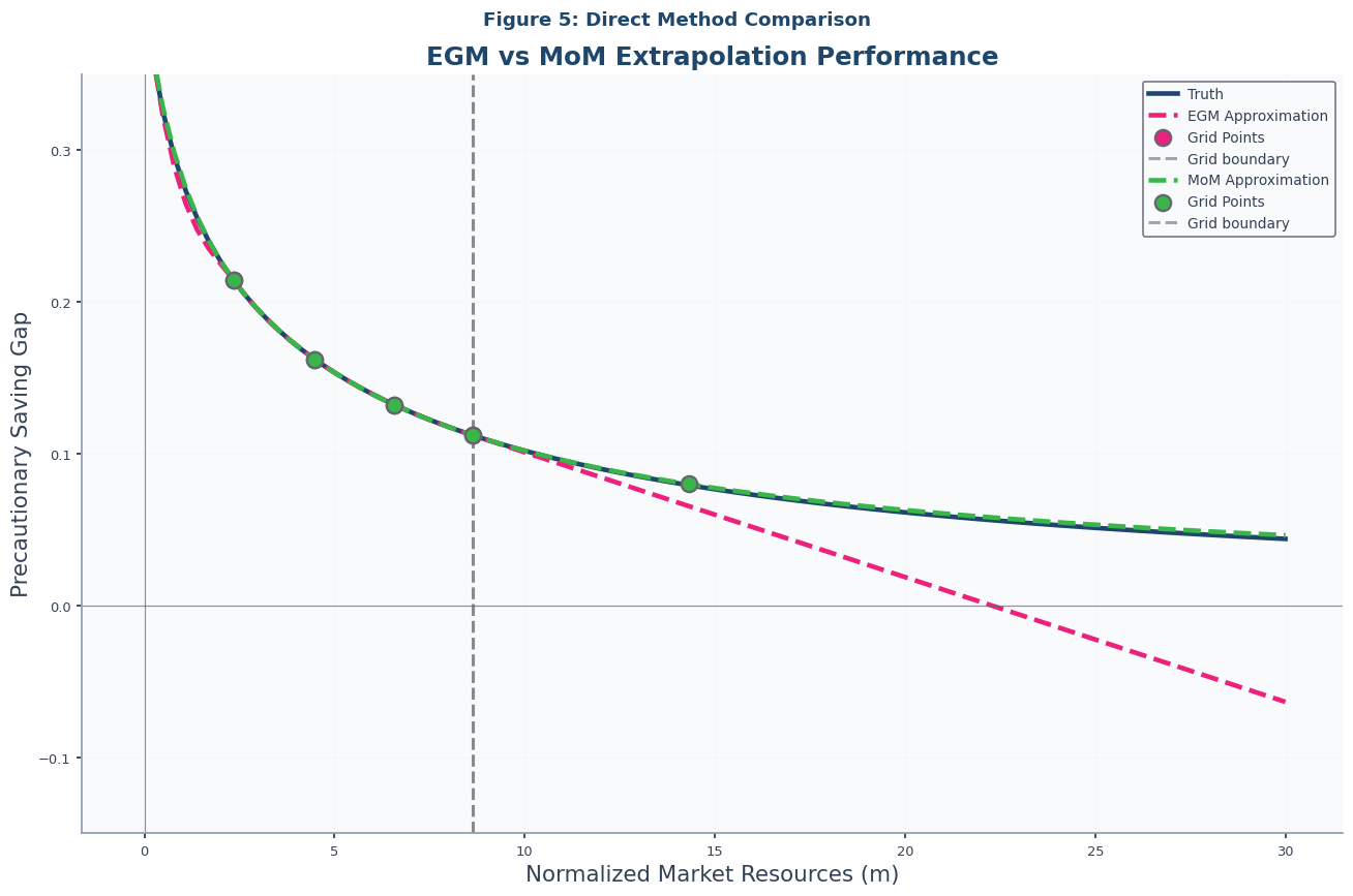
Figure 5: Direct Method Comparison¶

Notebook-code compares EGM and MoM precautionary gaps against the high-precision truth. Both approximations use identical 5-point sparse grids; the difference in extrapolation behavior is attributable solely to the method.

# Figure 5: Direct Method Comparison
plot_precautionary_gaps(
    truth_solution=IndShockTruthSol,
    approx_solutions=[IndShockEGMApproxSol, IndShockMoMApproxSol],
    title="Figure 5: Direct Method Comparison",
    subtitle="EGM vs MoM Extrapolation Performance",
)

Method of Moderation Framework¶

Figure 6: Moderation Ratio Function $\modRte(\mNrm)$ ¶

# Figure 6: Moderation Ratio Function
plot_moderation_ratio(
    solution=IndShockMoMApproxSol,
    title=r"Figure 6: Consumption Moderation Ratio $\omega(m)$",
    subtitle="Wealth-Dependent Moderation Between Bounds",
    m_max=50,
    grid_type=GridType.CONSUMPTION,
)

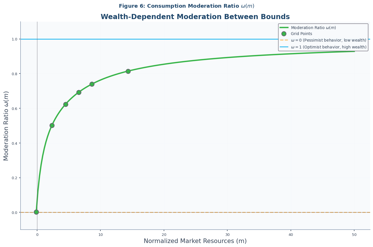
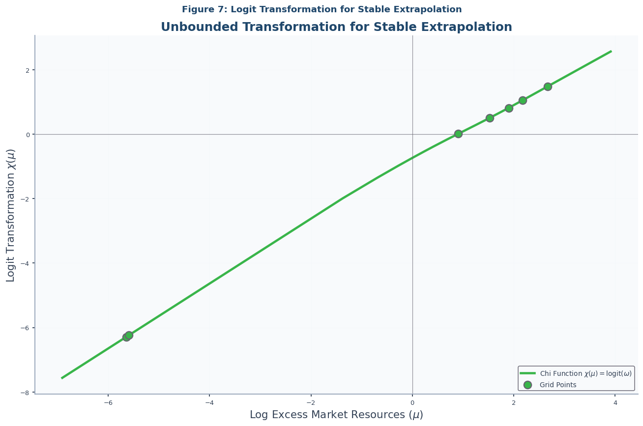
Figure 7: The Logit Transformation¶

# Figure 7: Logit Transformation Function
plot_logit_function(
    solution=IndShockMoMApproxSol,
    title="Figure 7: Logit Transformation for Stable Extrapolation",
    subtitle="Unbounded Transformation for Stable Extrapolation",
    m_max=50,
)

Function Properties and Bounds¶

Figure 8: MoM MPC Bounded by Theory¶

The MPC ( $\partial \cNrm / \partial \mNrm$ ) is bounded between $\MPCmin$ (optimist) and $\MPCmax$ (at the borrowing constraint), as detailed in the paper and Eq. (15) Carroll, 2001. Notebook-code confirms MoM respects these bounds.

# Figure 8: MoM MPC Bounds
plot_mom_mpc(
    solution=IndShockMoMApproxSol,
    title="Figure 8: MoM MPC Bounded by Theory",
    subtitle="MoM MPC Stays Within Theoretical Bounds",
)

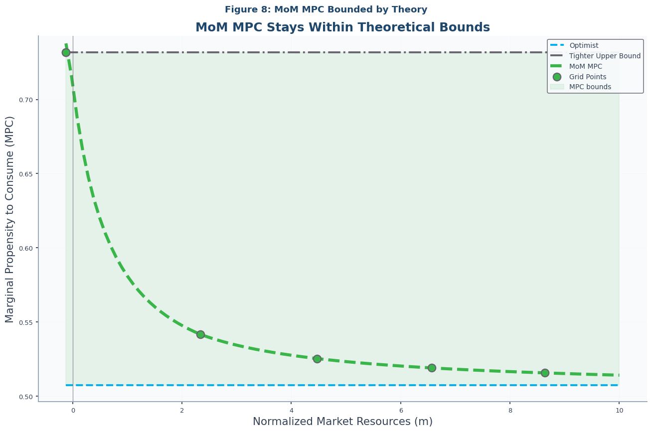
Figure 9: Value Functions Bounded by Theory¶

The value function $\vFunc(\mNrm)$ is also bounded by optimist and pessimist solutions Aiyagari, 1994Huggett, 1993. Notebook-code compares truth, EGM, and MoM value functions.

# Figure 9: Value Functions
plot_value_functions(
    truth_solution=IndShockTruthSol,
    title="Figure 9: Value Functions Bounded by Economic Theory",
    subtitle="Value Function: True Solution vs Sparse Approximations",
    egm_solution=IndShockEGMApproxSol,
    mom_solution=IndShockMoMApproxSol,
)

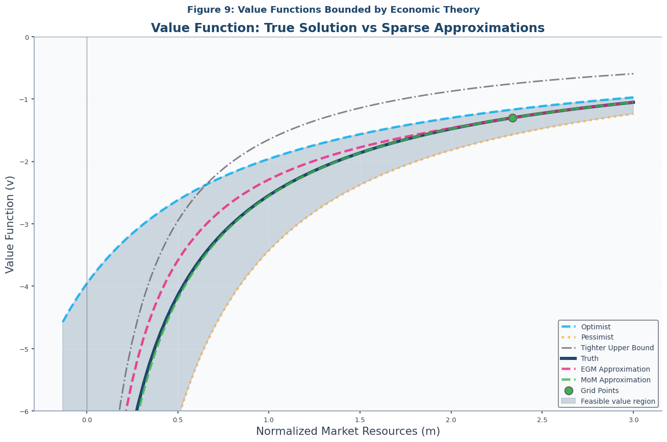
Figure 10: Inverse Value Functions $\vInv(\mNrm)$ ¶

The inverse value function $\vInv(\mNrm) = \uFunc^{-1}(\vFunc(\mNrm))$ gives the consumption equivalent of lifetime utility. It is more linear than $\vFunc(\mNrm)$ near the borrowing constraint, making it better suited for interpolation. Notebook-code compares the three solutions.

# Figure 10: Inverse Value Functions
plot_value_functions(
    truth_solution=IndShockTruthSol,
    title="Figure 10: Inverse Value Functions",
    subtitle="Inverse Value Function: Consumption-Equivalent Utility",
    inverse=True,
    egm_solution=IndShockEGMApproxSol,
    mom_solution=IndShockMoMApproxSol,
)

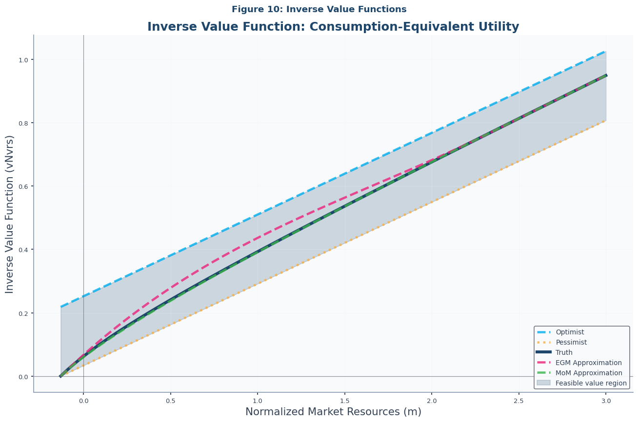
Figure 11: Value Function Moderation Ratio¶

MoM applies to any bounded function. The inverse value function moderation ratio (Eq. (9)):

\valModRte(\mNrm) = \frac{\vInvReal(\mNrm) - \vInvPes(\mNrm)}{\vInvOpt(\mNrm) - \vInvPes(\mNrm)}

(3)

follows the same pattern as the consumption ratio, as shown in Notebook-code.

# Figure 11: Value Function Moderation Ratio
plot_moderation_ratio(
    solution=IndShockMoMApproxSol,
    title=r"Figure 11: Value Function Moderation Ratio $\Omega(m)$",
    subtitle="Value Function Moderation Between Bounds",
    m_max=10,
    grid_type=GridType.VALUE,
)

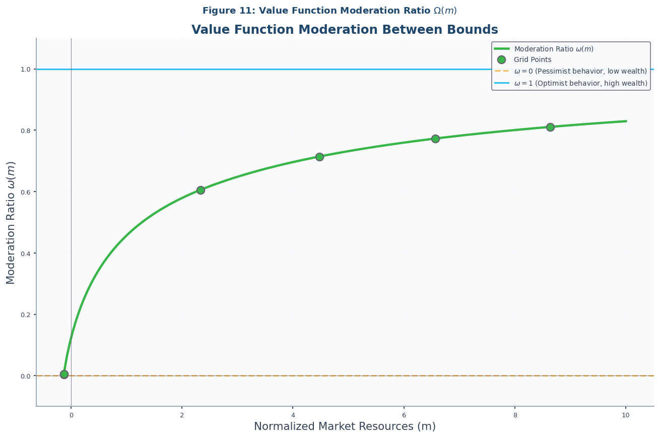
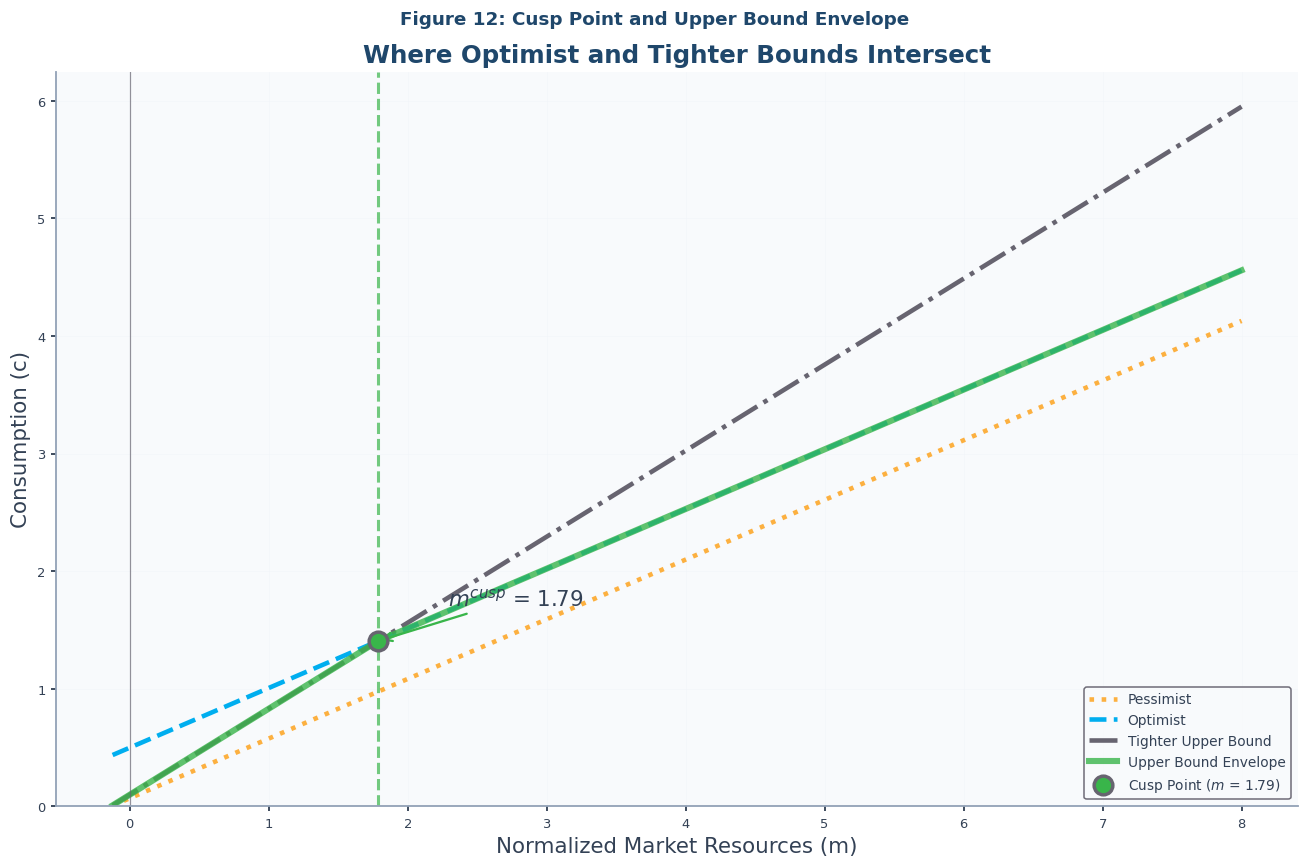
Figure 12: Cusp Point Visualization¶

The cusp point (Eq. (12)) is where optimist and tighter upper bounds intersect:

\mNrmCusp = \mNrmMin + \frac{\MPCmin \cdot \hNrmEx}{\MPCmax - \MPCmin}

(4)

Below the cusp, the tighter bound ( $\MPCmax$ slope) constrains; above, the optimist bound constrains. See IndShockMoMCuspConsumerType for the three-piece implementation.

# Figure 12: Cusp Point Visualization
plot_cusp_point(
    solution=IndShockMoMApproxSol,
    title="Figure 12: Cusp Point and Upper Bound Envelope",
    subtitle="Where Optimist and Tighter Bounds Intersect",
    m_max=8,
)

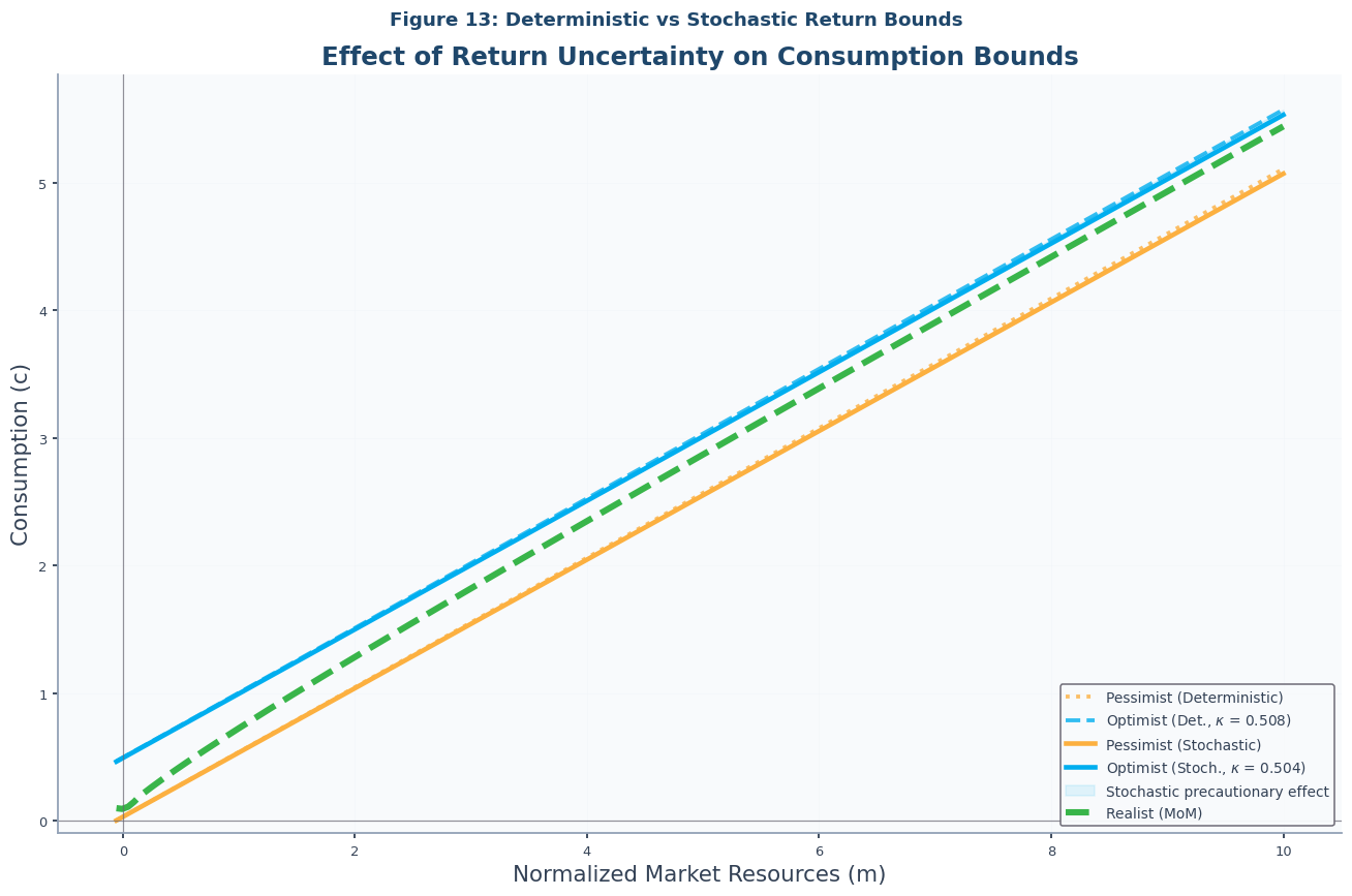
Further Extensions: Stochastic Rate of Return¶

With i.i.d. returns, Samuelson (1969) and Merton (1969)Merton (1971) show the consumption function remains linear for consumers without labor income. MoM extends directly by substituting the stochastic-return MPC Benhabib et al., 2018Carroll, 2020. Serially correlated returns remain for future research.

Figure 13: Stochastic Returns Comparison¶

Notebook-code compares bounds under deterministic and stochastic returns using IndShockMoMStochasticRConsumerType.

# Solve model with stochastic returns (mean-preserving spread)
stoch_params = params.copy()
stoch_params["RiskyAvg"] = params["Rfree"][0]  # Same mean as Rfree (scalar)
stoch_params["RiskyStd"] = (
    0.20  # 20% standard deviation (must satisfy β*E[R^{1-ρ}] < 1)
)

IndShockStochR = IndShockMoMStochasticRConsumerType(**stoch_params)
IndShockStochR.solve()
IndShockStochRSol = IndShockStochR.solution[0]

# Figure 13: Stochastic Returns Comparison
plot_stochastic_bounds(
    solution=IndShockStochRSol,
    title="Figure 13: Deterministic vs Stochastic Return Bounds",
    subtitle="Effect of Return Uncertainty on Consumption Bounds",
    m_max=10,
)

Summary¶

MoM solves the extrapolation problem by interpolating a moderation ratio via an asymptotically linear logit transformation, ensuring solutions respect theoretical bounds by construction.

Key Advantages:

Theoretical Consistency: Prevents negative precautionary saving.
Numerical Stability: Robust solutions via bounded transformations.
Computational Efficiency: Builds on EGM with minimal overhead.

For complete theoretical development see The Method of Moderation.

References¶

Friedman, M. (1957). A Theory of the Consumption Function. Princeton University Press.
Muth, J. F. (1960). Optimal Properties of Exponentially Weighted Forecasts. Journal of the American Statistical Association, 55(290), 299–306. 10.1080/01621459.1960.10482064
Carroll, C. D. (2020). Solving microeconomic dynamic stochastic optimization problems [Techreport]. Johns Hopkins University. https://www.econ2.jhu.edu/people/ccarroll/SolvingMicroDSOPs.pdf
Leland, H. E. (1968). Saving and Uncertainty: The Precautionary Demand for Saving. Quarterly Journal of Economics, 82(3), 465–473. 10.2307/1879518
Sandmo, A. (1970). The Effect of Uncertainty on Saving Decisions. Review of Economic Studies, 37(3), 353–360. 10.2307/2296725
Kimball, M. S. (1990). Precautionary Saving in the Small and in the Large. Econometrica, 58(1), 53–73. 10.2307/2938334
Carroll, C. D. (1997). Buffer-Stock Saving and the Life Cycle/Permanent Income Hypothesis. Quarterly Journal of Economics, 112(1), 1–55. 10.1162/003355397555109
Stachurski, J., & Toda, A. A. (2019). An Impossibility Theorem for Wealth in Heterogeneous-Agent Models. Journal of Economic Theory, 182, 1–24. 10.1016/j.jet.2019.04.001
Ma, Q., Stachurski, J., & Toda, A. A. (2020). The Income Fluctuation Problem and the Evolution of Wealth. Journal of Economic Theory, 187, 105003. 10.1016/j.jet.2020.105003
Carroll, C. D. (2006). The method of endogenous gridpoints for solving dynamic stochastic optimization problems. Economics Letters, 91(3), 312–320. 10.1016/j.econlet.2005.09.013
Barillas, F., & Fernández-Villaverde, J. (2007). A Generalization of the Endogenous Grid Method. Journal of Economic Dynamics and Control, 31(8), 2698–2712. 10.1016/j.jedc.2006.08.005
Hintermaier, T., & Koeniger, W. (2010). The Method of Endogenous Gridpoints with Occasionally Binding Constraints among Endogenous Variables. Journal of Economic Dynamics and Control, 34(10), 2074–2088. 10.1016/j.jedc.2010.05.002
Fella, G. (2014). A Generalized Endogenous Grid Method for Non-smooth and Non-concave Problems. Review of Economic Dynamics, 17(2), 329–344. 10.1016/j.red.2013.07.001
Iskhakov, F., Jørgensen, T. H., Rust, J., & Schjerning, B. (2017). The Endogenous Grid Method for Discrete–Continuous Dynamic Choice Models with (or without) Taste Shocks. Quantitative Economics, 8(2), 317–365. 10.3982/qe643
White, M. N. (2015). The Method of Endogenous Gridpoints in Theory and Practice. Journal of Economic Dynamics and Control, 60, 26–41. 10.1016/j.jedc.2015.08.001

The Method of Moderation: Illustrative Notebook

The Method of Moderation: Illustrative Notebook¶

Model Foundations: The Friedman-Muth Income Process¶

The Extrapolation Problem in Consumption-Saving Models¶

Consumption Function Analysis¶

Figure 1: The EGM Extrapolation Problem¶

Figure 2: Truth Bounded by Theory¶

Figure 3: Method of Moderation Solution¶

Figure 4: MoM Consumption Function¶

Figure 5: Direct Method Comparison¶

Method of Moderation Framework¶

Figure 6: Moderation Ratio Function ω(m)\modRte(\mNrm)ω(m)¶

Figure 7: The Logit Transformation¶

Function Properties and Bounds¶

Figure 8: MoM MPC Bounded by Theory¶

Figure 9: Value Functions Bounded by Theory¶

Figure 10: Inverse Value Functions Λ(m)\vInv(\mNrm)Λ(m)¶

Figure 11: Value Function Moderation Ratio¶

Figure 12: Cusp Point Visualization¶

Further Extensions: Stochastic Rate of Return¶

Figure 13: Stochastic Returns Comparison¶

Summary¶

Figure 6: Moderation Ratio Function $\modRte(\mNrm)$ ¶

Figure 10: Inverse Value Functions $\vInv(\mNrm)$ ¶